Date: February 26, 2020 (Concept Check, Class Responses, Solutions)

Relevant Textbook Sections: 4.4

Cube: Supervised, Discrete or Continuous, Nonprobabilistic

Lecture 9 Summary

• Intro: More Context and Examples of Neural Networks
• Optimizing the Neural Network
• Detour: Vector Chain Rule
• Let's Now Finish The Optimization
• Let's Generalize Everything
• Why does this all work?

Intro: More Context and Examples of Neural Networks

Last lecture, we described different neural network models and architectures. Today, we will be focusing on the optimization of neural networks. These are going to be difficult, but will be important to understand.

Also, before we move on, let's cover a few more examples of the use of neural networks. One thing we can do now is predict the aftershocks of earthquakes extremely efficiently using neural networks. Before, we had to use physics data to run the simluation to understand what is going to be expected, but now we can instead use a neural network on the data, and it's about as accurate. Another example is the creation of blue LED's. It's incredibly expensive to make these lights, as you have to make them, test them, and this can cost thousands of dollars. Now, we can predict which molecules are the most likely to be effective at creating the blue LED lights. Basically, at a cheaper cost, and in a shorter time, we'll be able to find a good molecule for this purpose, and create blue LED lights much more effective. This is a great example of an intersection of engineering and machine learning.

Optimizing the Neural Network

As usual, just as what we've done a long time ago, after we've picked our model class, and after we've picked our loss function (which we will do down below), we will need to optimize our loss function with respect to our parameters to solve for our final model.

Ultimately, we want this specifically:

$$\frac{\partial L_n}{\partial W}$$ To think through this, we know that we can do this because within the loss function, we'll be including the $f_n$ (see diagram from last lecture for context if you don't remeber what this is) term, and within the $f_n$ term, we can ultimately take the gradient with respect to W. We can use the chain rule to depict this:

$$\frac{\partial L_n}{\partial W} = \frac{\partial L_n}{\partial f_n} \frac{\partial f_n}{\partial W}$$ The reason discuss this intuition first is to give context for what we're about to do below. As you can see, essentially to calculate $\frac{\partial L_n}{\partial W}$, we are going to take many steps, and one of the steps we can take first is to find the $\frac{\partial L_n}{\partial f_n}$, which we will do below for two different example loss functions. It is also important to note that this part of the equation is independent of the other derivatives, so it is totally fair game to calculate this first.

Also in lecture today, we will cover back propagation, which relates very much to the above equation. To paraphrase Wikipedia (which I think has a great explanation): The concept of backpropagation is that we will compute the gradient of the loss (with respect to the weights) in an efficient way, which makes training networks with multiply layers actually possible. Specifically, back propagation is computing the gradient of the loss function a layer at a time, starting from the final layer (and going backwards), and then resuing terms so that we don't have to repeat any calculations (for intermediate terms in the chain rule). If you've taken CS124, this is an example of dynamic programming!

Even though in real life, we probably will use packages to implement this and not implement backpropagation ourselves, it's good to understand the intuition behind this so we can better use the tools availble to us. By underestanding the details, we will know why are certain things slower, and why are certain things faster, etc.

Loss Function (if regression)

First, let's define an example loss function that we might use for regression (note: we can always choose other loss functions for regression as well, it doesn't have to be least squares). Below, we have the least squares loss. Just a note, we will be as general as possible, and hence are splitting up the notes into this format of regression and classification. Also note, where we used to put in $\hat{y}$ in linear regression in the past, now we're putting in $f_n$. $$L(w) = 1/2 * \sum(y_n - f_n)^2$$ Let us take the derivative:

$$dL/df_n = \sum_n (y_n - f_n)(-1)$$ Note: If we swapped it to another loss function, we also note that the only effect on the whole original expression $\frac{\partial L_n}{\partial W}$ is only in this specific part, $\frac{\partial L_n}{\partial f_n}$.

Loss Function (if classification)

As mentioned before, we are being as general as possible, so we also write here a loss function for classification, as another example. Let's pick the logistic loss here as our example.

Remember first that for our binary classification, we define the following:

$$p(y=1|x) = \sigma(f_n)$$ $$p(y=0|x) = 1 - \sigma(f_n)$$ Now, we can define the logistic loss function using the terms above:

$$L(w) = \sum_n y_n \log p(y=1|x) + (1 - y_n) \log p(y=0|x)$$ $$L(w) = \sum_n y_n \log \sigma(f_n) + (1 - y_n) \log (1 - \sigma(f_n))$$ Also remember the following helpful tip for the derivative:

$$\frac{\partial\sigma(z)}{z} = \sigma(z)(1 - \sigma(z))$$ Let us take the derivative:

$$\frac{\partial L_n}{\partial f_n} = y_n \frac{1}{\sigma(f_n)} \sigma(f_n) (1 - \sigma(f_n)) + (1 - y_n) \frac{1}{1 - \sigma(f_n)} \sigma(f_n)(1 - \sigma(f_n))(-1)$$ We can simplify:

$$\frac{\partial L_n}{\partial f_n} = y_n (1 - \sigma(f_n)) - (1 - y_n) \sigma(f_n)$$

Detour: Vector Chain Rule

We will take a slight detour now in order to gain the tools we need to do the back propagation. $$y = f(u) = f(g(h(x)))$$ $$u = g(v) = g(h(x))$$ $$v = h(x)$$

All Scalars

If we had all scalars, and we wanted to look for: $\frac{\partial f}{\partial x}$

$$\frac{\partial f}{\partial x} = \frac{\partial f}{\partial u}\frac{\partial u}{\partial v} \frac{\partial v}{\partial x} = \frac{\partial f}{\partial u}\frac{\partial g}{\partial v}\frac{\partial h}{\partial x}$$

If x (size $D$) was a vector

$$\nabla_\mathbf{x}f = \frac{\partial f}{\partial u} \frac{\partial u}{\partial v} \nabla_\mathbf{x}v$$ Where $\frac{\partial f}{\partial u} and \frac{\partial u}{\partial v}$ parts scalar, and $\nabla_\mathbf{x} v$ is $1 \times D$ a vector: as in how does each dimension of $\mathbf{x}$ affect scalar $v$.

Note: We are using the numerator layout notation (sometimes known as the Jacobian formulation), where $\mathbf{y}$ and $\mathbf{x}$ are size $M$ and $N$ vectors respectively and $\frac{\partial \mathbf{y}}{\partial \mathbf{x}}$ is an $M\times N$ matrix such that $$\frac{\partial \mathbf{y}}{\partial \mathbf{x}} = \begin{pmatrix} \frac{\partial y_1}{\partial x_1} & \frac{\partial y_1}{\partial x_2} & \cdots & \frac{\partial y_1}{\partial x_N} \\ \frac{\partial y_2}{\partial x_1} & \frac{\partial y_2}{\partial x_2} & \cdots & \frac{\partial y_2}{\partial x_N} \\ \vdots & \vdots & \ddots & \vdots \\ \frac{\partial y_M}{\partial x_1} & \frac{\partial y_M}{\partial x_2} & \cdots & \frac{\partial y_M}{\partial x_N} \end{pmatrix}$$ $\frac{\partial \mathbf{y}}{\partial \mathbf{x}}$ is known as the Jacobian matrix and represented as $\mathbb{J}_\mathbf{x}[\mathbf{y}]$.

If x (size $D$) and v (size $J$) were both vectors

$$\nabla_\mathbf{x} f = \frac{\partial f}{\partial u} \nabla_\mathbf{v}u \mathbb{J}_\mathbf{x}[\mathbf{v}]$$ $\frac{\partial f}{\partial u}$ is a scalar, $\nabla_\mathbf{v}u$ is a $1 \times J$ vector, and $\mathbb{J}_\mathbf{x}[\mathbf{v}]$ is a $J \times D$ matrix.
$\mathbb{J}_\mathbf{x}[\mathbf{v}]$ measures how each dimension of $\mathbf{x}$ affects each dimension of $\mathbf{v}$ and $\nabla_\mathbf{v}u$ how each dimension of $\mathbf{v}$ affects each dimension of $u$.
Chaining them, $\nabla_\mathbf{v}u \mathbb{J}_\mathbf{x}[\mathbf{v}]$ ($1 \times D$ vector) measures how each dimension of $\mathbf{x}$ affects each dimension of $u$.
Consequentially, $\frac{\partial f}{\partial u} \nabla_\mathbf{v}u \mathbb{J}_\mathbf{x}[\mathbf{v}]$ is a vector of how each $\mathbf{x}$ dimension changes scalar $f$, through all dimensions of $\mathbf{v}$ and $u$.

If x (size $D$) and v (size $J$) and u (size $J^\prime$) were all vectors

$$\nabla_\mathbf{x} f = \nabla_\mathbf{u} f \mathbb{J}_\mathbf{v}[\mathbf{u}] \mathbb{J}_\mathbf{x}[\mathbf{v}]$$ $\nabla_\mathbf{u} f$ is a $1 \times J^\prime$ vector, $\mathbb{J}_\mathbf{v}[\mathbf{u}]$ is a $J^\prime \times J$ matrix, $\mathbb{J}_\mathbf{x}[\mathbf{v}]$ is a $J\times D$ matrix. We still get a vector of how each $\mathbf{x}$ dimension changes scalar $f$, through all dimensions of $\mathbf{v}$ and $\mathbf{u}$.

Let's Now Finish The Optimization

As a refresher, we've had from before: $$\frac{\partial L_n}{\partial \mathbf{w}} = \frac{\partial L_n}{\partial f_n} \frac{\partial f_n}{\partial \mathbf{w}}$$ We already calculated $\frac{\partial L_n}{\partial f_n}$ before, so we need to now calculate $\frac{\partial f_n}{\partial \mathbf{w}}$. Let's say our $f_n = \mathbf{w}^T\mathbf{\phi_n} + b$. If so, that means we have: $$\frac{\partial f_n}{\partial \mathbf{w}} = \mathbf{\phi_n}$$

Example: Let's Complete the Full Expression for the Regression Case

From before for the regression case, we have $\frac{\partial L_n}{\partial f_n} = (y_n - f_n)(-1)$, and now we have $\frac{\partial f_n}{\partial \mathbf{w}} = \mathbf{\phi_n}$, so combined we have:

$$\frac{\partial L_n}{\partial \mathbf{w}} = (y_n - f_n)(-1) \mathbf{\phi_n}$$

Notice that we need the value $f_n$ to compute the gradient.
How will we get this term? We can first compute $\mathbf{x} \rightarrow \mathbf{\phi_n} \rightarrow \mathbf{f_n}$ and then use that value of $\mathbf{f_n}$ in the gradient.

Recall that $\mathbf{\phi_n} = \sigma (\mathbf{W}^1\mathbf{x} + \mathbf{b}^1)$. How can we get $\nabla_\mathbf{W}\mathcal{L}_n$?

$$\nabla_\mathbf{W}\mathcal{L}_n = \frac{\partial L_n}{\partial f_n} \nabla_\mathbf{\phi_n}f_n \mathbb{J}_\mathbf{W}[\mathbf{\phi_n}]$$

Let's Generalize Everything

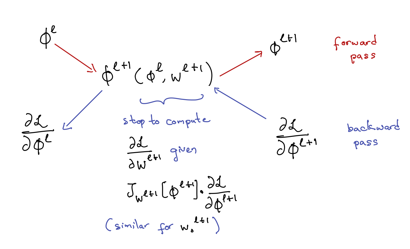
The process of computing gradients for optimizing neural networks is as follows:

1. Compute $\mathcal{L}(\mathbf{\phi}^{L}(\mathbf{\phi}^{L-1}(\cdots \mathbf{\phi}^{1}(\mathbf{x}))))$ by passing $\mathbf{x}$ through the network $\mathbf{x} \rightarrow \mathbf{\phi}^{1} \rightarrow \cdots \rightarrow \mathbf{\phi}^{L-1} \rightarrow \mathbf{\phi}^{L} \rightarrow \mathcal{L}$ (this is called a forward pass) and store all $\mathbf{\phi}^\ell$.
2. Perform the chain-rule backwards:
   • $$\frac{\partial \mathcal{L}}{\partial \mathbf{\phi}^\ell} = \nabla_{\mathbf{\phi}^L}\mathcal{L} \mathbb{J}_{\mathbf{\phi}^{L-1}}[\mathbf{\phi}^{L}] \cdots \mathbb{J}_{\mathbf{\phi}^{\ell}}[\mathbf{\phi}^{\ell + 1}]$$
   • Compute the parameter gradients $$\begin{align*} \frac{\partial \mathcal{L}}{\partial \mathbf{W}^\ell} &= \nabla_{\mathbf{\phi}^L}\mathcal{L} \mathbb{J}_{\mathbf{\phi}^{L-1}}[\mathbf{\phi}^{L}] \cdots \mathbb{J}_{\mathbf{\phi}^{\ell}}[\mathbf{\phi}^{\ell + 1}] \mathbb{J}_{\mathbf{W}^{\ell}}[\mathbf{\phi}^{\ell}] \\ &= \frac{\partial \mathcal{L}}{\partial \mathbf{\phi}^\ell} \frac{\partial \mathbf{\phi}^\ell}{\partial \mathbf{W}^\ell} \end{align*}$$

The following picture shows the steps

Note: This is called "reverse-mode" autodiff. This is good when the output ($y$) is small and there are many parameters (all the $W$s). It allows for efficient reuse of computed values.

We can also do "forward-mode" diff. Suppose we wanted just a derivative/sensitivity test on $\frac{\partial \mathcal{L}_n}{\partial x_{nd}}$. Then we don't need all the $\frac{\partial \mathbb{\phi}}{\partial W_{jd^\prime}}$ for all $d^\prime \neq d$.
Forward mode goes from the variable $x_{nd}$ to $\mathcal{L}_n$ rather than from $\mathcal{L}_n$ to $x_{nd}$.
We compute $\frac{\partial \mathbf{\phi}^1}{\partial x_{nd}}$, then $\frac{\partial \mathbf{\phi}^2}{\partial \mathbf{\phi}^1}$ all the way up.

Why does this all work?

1. GPUs allow fast computations of linear algebra
2. We now have lots of data, and lots of data avoids overfitting
3. Practicalities
   • Theory is lagging, but belief is that the over-parameterization enables easier gradient descent (gradient descent doesn't work in simpler models)
   • Tricks: perturb inputs to avoid overfitting, stop when validation loss increases (potentially), L1 and L2 Regularization