Date: April 8, 2020 (Lecture Video, iPad Notes, Concept Check, Class Responses, Solutions)

Lecture 18 Summary

• Intro: Another Example of Bayesian Networks
• Setting it Up
• Specific Example of Inference
• Back to Original Setup: Choosing the Order of Elimination
• What does the min cost of inference depend on?
• How to get Optimal Order for Polytrees
• Preview to Next Lecture: Hidden Markov Models
• Final Notes

Intro: Another Example of Bayesian Networks

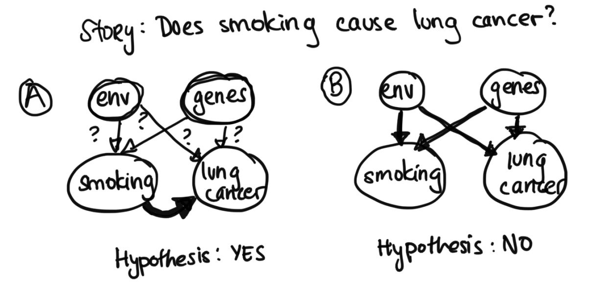
Last time, we defined Bayesian Networks, and we saw how they are useful in the probabilistic setting regardless of whether we're in the unsupervised or superivsed world, as it helps us describe structure in the data Today, we will cover how to do inference in Bayesian netowrks.

Before moving on, we'll look at a real world application of Bayes Nets. While nowadays most people know that smoking is damaging to the lungs, in the past, this was an open question. Because we couldn't do a randomized trial where we made one group smoke and another group not (due to ethical concerns), we were never able to tell the difference between correlation and causation. Even though it looked like the rate of lung cancer is higher in smokers than nonsmokers, tobacco companies and other argued that perhaps the same genes lead to people getting lung cancer and wanting to smoke. Or, perhaps growing up in a certain enviroment causes both the lung caner and an increased likelihood to smoke. Does smoking actually cause lung cancer? It was impossible to tell (see diagram below, for the two hypotheses in Bayes Nets Form).

In history, how we ended up resolving this was that researchers actually found carcinogens through testing smoking with animals, and so ultimately the debate was resolved that way. But actually, here we could also check this hypothesis using Bayes Nets. Given environment and genes, we could figure out whether smoking and lung cancer were still independent in the data. If yes, then fair, we can't draw any conclusions about smoking and lung cancer. But if no, we could rule out the conclusions the envrionment and/or genes were causing both smoking and lung cancer together. Unfortunately, at the time, the exact data necessary on smoking was not available yet, and hence this debate was resolved in the other manner. But if it hadn't been resolved yet, and that data is available like it is now, then this is a great example of how we can use Bayes Nets to help us reason through the problem.

Setting it Up

Let's say we have this following setup.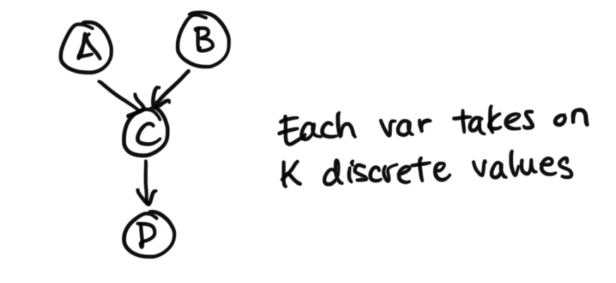
Before we go through anything else in lecture, let's first just look at finding p(D), which which will be a vector of probabilities for each of the K possible value of D (since we said it's discrete). We can do the following: $$p(D) = \sum_{A, B, C} p(A, B, C, D)$$ $$p(D) = \sum^K_{A=1} \sum^K_{B=1} \sum^K_{C=1} p(A) p(B) p(C | B, A) p(D | C)$$ This is just a general property to keep in mind without doing anything special. Specifically, in order to do the above computation, for each value of D (where there are K of them), we would need to sum out K values of A, B, and C, which would lead to $K^4$ computational steps in total. We get this idea in our minds first as we move on, because later in lecture we will do some tricks to make the computation easier.

Specific Example of Inference

Let's try the following example, involving rain, a sprinkler, and wet grass: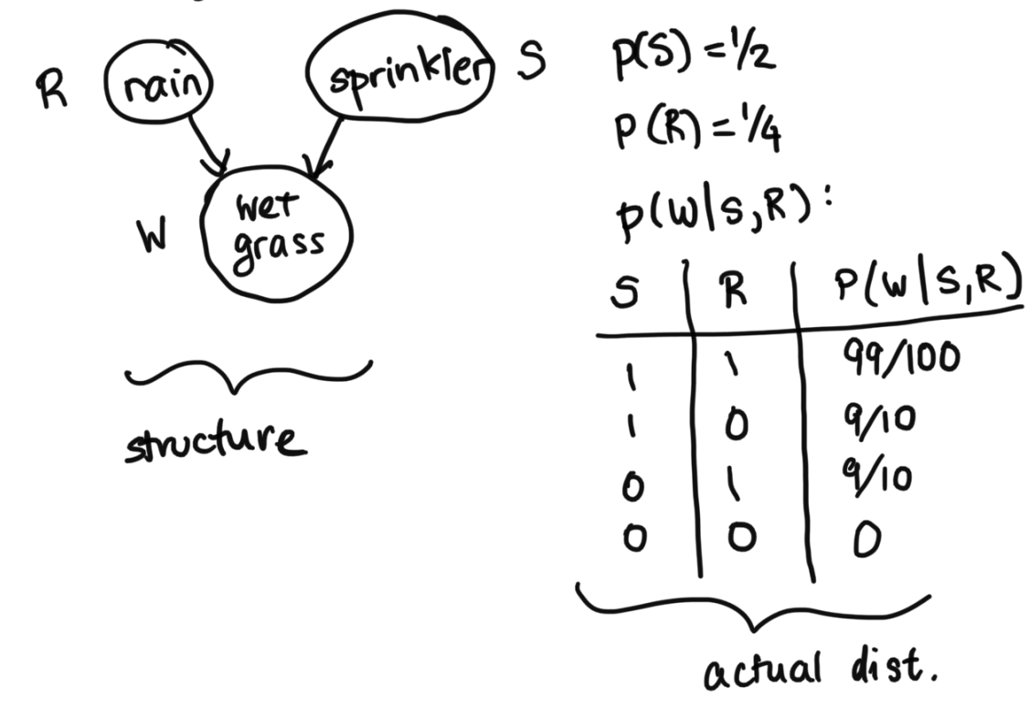 We have the structure on the left, and we have the actual dstribution on the right. So farh, this is just a refresher from last class. Now, let's do some inference. Suppose we were looking for:

Find the Probability It Rained Given Wet

Let's say we're looking to infer what the probability it rained given that we have observed that the grass is wet. $$p(R=1 | W=1) = \frac{p(R=1, W=1)}{p(W=1)}$$ $$p(R=1 | W=1) = \frac{p(R=1, W=1)}{p(R=1, W=1) + p(R=0, W=1)}$$ In order to do this, we actually have to break it down. This is exact same concept as what we wrote above in the section above, where we said we would have to sum over A, B, C. Here, because we don't know what happened with the sprinkler, we will have to sum over the different possibilities for the sprinkler. $$p(R=1 | W=1) = \frac{p(R=1, W=1, S=0) + p(R=1, W=1, S=1)}{p(R=1, W=1, S=0) + p(R=1, W=1, S=1) + p(R=0, W=1, S=0) + p(R=0, W=1, S=1)}$$ To make things concrete, we break down these values in detail: $$p(R=1, W=1, S=0) = p(R=1) p(S=1) p(W=1 | S=0, R=1) = (1/4)(1/2)(9/10)$$ $$p(R=1, W=1, S=1) = p(R=1) p(S=1) p(W=1 | S=1, R=1) = (1/4)(1/2)(99/100)$$ $$p(R=0, W=1, S=0) = p(R=0) p(S=1) p(W=1 | S=0, R=0) = (3/4)(1/2)(0)$$ $$p(R=0, W=1, S=1) = p(R=0) p(S=1) p(W=1 | S=1, R=0) = (3/4)(1/2)(9/10)$$ $$p(R=1 | W=1) = \frac{(1/4)(1/2)(9/10) + (1/4)(1/2)(99/100)}{(1/4)(1/2)(9/10) + (1/4)(1/2)(99/100) + (3/4)(1/2)(0) + (3/4)(1/2)(9/10)} = 21/51 = 0.41176$$ Recall that: $$p(R) = 0.25$$ This shows us how, if the grass is wet, the probability of rain has increased, from our prior of 0.25 to 0.41176 which makes sense intuitively. If the grass is wet, it's probably a bit more likely that it rained.

Find the Probability it Rained given Wet and Sprinkler On

Now, let's add a dimension of information in. What if besides the fact that the grass is wet, we also knew that the sprinkler was on. Intuitively, we should now get a lower probbility that it rained, because the sprinkler being on helps explain why the grass is wet. Let's make sure the math checks out: $$p(R=1 | W=1, S=1) = \frac{p(R=1, W=1, S=1)}{p(W=1, S=1)} = \frac{p(R=1, W=1, S=1)}{p(R=1, W=1, S=1) + p(R=0, W=1, S=1)}$$ $$p(R=1 | W=1, S=1) = \frac{(1/4)(1/2)(99/100)}{(1/4)(1/2)(99/100) + (3/4)(1/2)(9/10)} = 11/41 = 0.26829$$ This is indeed lower, and is now closeer back to the prior of 0.25. Again, this makes sense, because we also saw that the sprinklers were on (in addition to the grass being wet), which reduces the chances that it has rained, since the sprinkler has helped explain the grass has been wet. This is called the explaining away effect. It refers to one of the d separation rules we covered in last lecture.

Find the Probability it Rained given Wet and Sprinkler Off

For a sanity check, let's look at the other case, p(R=1 | W=1, S=0). This should actually be 1, because we had set p(W=0 | S=0, R=0) to be 0, basically saying that if it didn't rain and the sprinkler was off, there's no way the grass was wet. So if we know for a fact that it wasn't the sprinkler that cuased it to be wet (since it's off), that it must've rained with probability 1. Let's make sure the math checks out: $$p(R=1 | W=1, S=0) = \frac{p(R=1, W=1, S=0)}{p(W=1, S=0)} = \frac{p(R=1, W=1, S=0)}{p(R=1, W=1, S=0) + p(R=0, W=1, S=0)}$$ $$p(R=1 | W=1, S=0)= \frac{(1/4)(1/2)(9/10)}{(1/4)(1/2)(9/10) + (3/4)(1/2)(0)} = \frac{(1/4)(1/2)(9/10)}{(1/4)(1/2)(9/10)} = 1$$

Back to Original Setup: Choosing the Order of Elimination

From before, we had the following diagram. From before, we noted that: $$p(D) = \sum_{A, B, C} p(A, B, C, D) = \sum^K_{A=1} \sum^K_{B=1} \sum^K_{C=1} p(A) p(B) p(C | B, A) p(D | C)$$ Which would cost $K^4$ steps of computation, if doing the most simple things. It turns out that we can actually rearrange the sum in the following way, and rearranging is called choosing the order of elimination (since we are eliminating variables out in a particular order now, not just randomly summing out the variables): $$\sum_C p(D|C) \sum_B p(B) \sum_A p(A) p(C | A, B)$$ We can start summing out the edges from the top moving down. So first, we'll sum out all the terms releavnt to A (which are p(A) and p(C|A, B) since A are involved in these terms).

As we do the sum over A, we notice that $p(C | A, B)$ is a cube of K by K by K numbers (since it has 2 children) and p(A) is a vector of size K. After the summation over A, we have a K by K quantity since we've summed out the A, but still have terms involving C and B, so we can rewrite this as a function g(C, B). We will have to deal with this at some point, but for now after summming out A we've turned this into a K by K quantity first.

As we do the sum over B, we notice that Vector B is of size K, and from before, g(c, b) is K by K. After the summation, we result in a new quantity g(c), which of just size K.

Finally, in the last sum, this gives the quantity of size K, the solution.

Note: this computation is now only $K^3$ (no longer $K^4$), which is way better. The reason is cause we only had to deal with the p(C|A, B) K by k by K cube term once. We compressed it into K by K right away, so the rest of the way we didn't have to deal with so many values. On the other hand, in the original method at the beginning of lecture, we had to deal with the cubed term over and over, leading to the $K^4$ computation.

Student Question: How do we sum up over A without any knowledge of B? This is a great question. When we sum over A, we are truly just eliminating A, so you're right, we don't know what B is. This is why in our resulting term g(c, b), it is still a function of B. Imagine we start with A B C, a cube of values. We're just summing over one dimension, the A, so we leave behind still a square which is B by C.

Important note: not all orders are necessarily better. We had our summations arranged in the order, $\sum_C \sum_B \sum_A$ which means we picked elminiating A, B, then C. If we had picked $\sum_A \sum_B \sum_C$ (also known as eliminating out C, then B, then A), we would still get $K^4$.

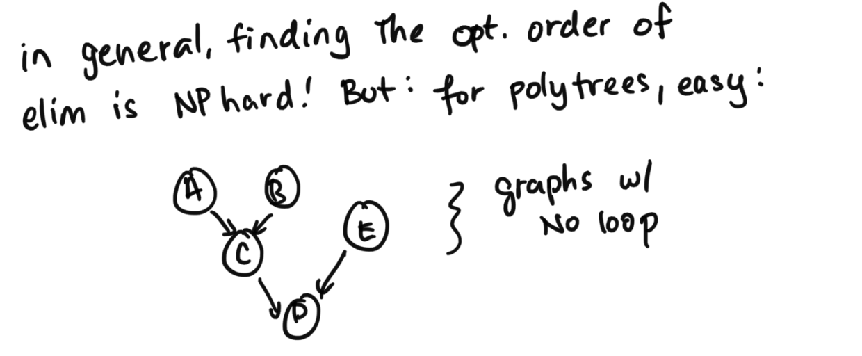
What does the min cost of inference depend on?

How do we determine the minimum cost of inference? This will depend on something called treewdith. One way to think about it is the maximum number of interacting variables. For us, our bottleneck was p(C|A, B), a triple dependency between variables. We definitely can't do anything better than that.

In general, finding the optimal order of elminatin is NP hard. But if we have a specific structure, polytrees specifically, it's easy. A polytree is a directed acyclic graph whose underlying undirected graph is a tree (which means the undirected graph is both connected and acyclic).

How to get Optimal Order for Polytrees

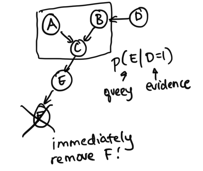
Step 1: Prune variables that are descenents of the queried or evidenced variables

First, we want to prune variables that are descendents of queries or evidence variables (also can be phrased as only keeping the ancestors of either). So when we are looking for p(B | A = 1), the query is B, evidence is A, and we can prune away C. To show this in the math, we can do the follwoing. $$p(B | A=1) = \sum_C p(B, A=1, C) = \sum p(B | A = 1) p(C | B) = p(B | A=1) \sum_C p(C|B)$$ The key is that $$\sum_C p(C|B) = 1$$, since we don't even care about C and when we sum over all the probabilities, it will just become 1. This formally shows in the math of why we can prune the descenedents (again, remember that this is only in the polytree situation).

Step 2: Find the leave and works backwards

Next, what is important is finding the leaves (ignoring the directions of the errors) and working backwards to the query. We'll use this new diagram for an example of this one. Say we're looking for p(E | D=1). First, we remove F immediately, as we learned from Step 1, since it's a descendent of E. Note: we can't remove B since even though it's a descendent of D, it's an acnestor of E. Next, we're going to focus on the variables we need to sum out (so we put the rectangle around A, B and C, since D and E are our evidence and query variables). We want to work from the edges in. So one option for the elimination order would be order, B, A, C. The other option would be A, B, C. They key point is that C is the last one in the order. Again, remember we are ignoring the directions of the arrows when looking for the leaves here. We have A and B as the leaves since they are just leaves off of C, but we need to make sure C is eliminated last because it's not a leaf and involves both A and B. These two steps will result in the most optimal order for polytrees!

Preview to Next Lecture: Hidden Markov Models

Let's look at a specific form of structure, the Hidden Markov Model, which is something we will cover next class.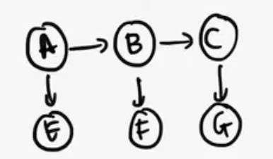 Why is this special structure interesting? This is interesting because you can imagine the top reprsents some time series of say a true location of what you're trying to track, like a plane, and E, F, G,correspond to radar measurements. When the plane was at A, the radar said it was at E, when the plane was at B, the radar said ti was at F, etc. Now, we want to know the probability of the current location of the plane given the last three sets of radar measurements. This is interesting because we never get to see A and B, but we get the condition on the measurements.

Let's say we have discrete values again, and we've observed our radar to tell us that E=1, F=1, and G=1. So let's say we're looking for p(C | E=1, F=1, G=1). $$p(C | E=1, F=1, G=1) = \sum_A \sum_B p(A) p(E=1|A) p(B|A) p(F=1|B) p(C|B) p(G=1|C)$$ How do we determine the proper order of elimination? Note that these are polytrees too. We also note, first of all there no descendents to be pruned away. Next, we see that for us to work from the leaves towards the query, so for us that means we want to eliminate A, then B (since A is furthest away from the query C). $$p(G=1|C) \sum_B p(F=1|B) p(C|B) \sum_A p(A) p(E=1|A) p(B|A)$$ As we sum out A, we notice that p(B|A) is K by K, and that after summing we will get a single vector K long, factor g(B).

As we sum out B, we know we will get another K size factor g(C).

These factors are often called "messages" (and you may see a message-passing algoirthm), which we will go into much more detail in the next class. But just to plant the seed first, the first factor g(B) is taking care of essentially the stuff in the past, because we know stuff about B with respect to the info from A and E. Then, the factor g(C), gives us the "message" about what's important from A, E, B and F. Again, more detail next class! The key idea is that in certain types of graphs, you can get some very specific patterns.

Note: What if we summmed it over a different way?

$$p(G=1|C) \sum_A p(A) p(E=1|A) \sum_B p(B|A) p(C|B) p(F=1|B)$$ As we sum out B, we see that all the terms inside, $p(B|A) p(C|B) p(F=1|B)$ is goign to be a K by K by K quantity (with, A, B, C), which will collapse to a factor g(A, C) after finishing the summing. Already, we notice that now we have something bigger than the other ordering.

As we sum out A, we will still have a g(C) vector.

Overall, we see that we have to store a K by K by K object and do the computation, so in terms of both computation and memory, the ordering from above is better.

Final Notes

There are really many algorithms for exact inference, but they're all the same ideas as what we covered today. It's good to know the other terminology out there so you can connect back to this.

• Sum-product (this is equivalent to exact inference, it's also called this because our equaitons are sums of products)
• Forward-backward (this is equivalent to the specific sum product idea for hidden markov models)
• Junction-tree (this occurs more in the theory litereature, and refers to specific type of tree structures like polytrees)

We can also move beyond exact inference for hard cases and do apprxomiate inference instead: using sampling-based methods, varational methods, etc. This is in case the graphs get really big, or if we are in continuous space then all the summations becomes integrals, which can be quite tricky. This isn't in the scope of 181, but Finale wanted to mention this for context (covered more in a class like 281).

Final Broader Note

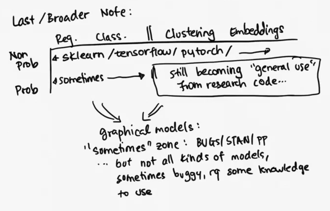
This final broader note is to help is situation ourselves in where we are back in the cube. We had nonprobablistic vs probablistic methods, and we had our supervised (regression vs classifiction) and unsupervised (clustering and embeddings) sides. On the nonprobablistic side, pretty much most things are 'solved', in th sense that using our favorite libraries, sklearn, tensorflow, pytorch, etc, we can do a pretty good job. On the probabilstic side, for supervised learning, we can also do this sometimes. However, on the probalistic unsuperivised side, the algorithms are still becoming "general use" from research code. These things aren't nearly as robust in this corner of the cube. If we look at graphical models in probabilisic settings, we're still in the "sometimes" zone, where there are some libraries out there such as BUGs and STand, and probablistic programming libaries, but not all kinds of models. They're sometimes buggy, and require some knowledge to use (not as simple as an sklearn call). If you want to use these things, there is code out there, but it's important to look at the code closely. Not completely related to today's topics, but important to note in the big picture sense about what the world of code looks like out there nowadays.