Date: April 15, 2020 (Lecture Video, iPad Notes, Concept Check, Class Responses, Solutions)
Lecture 20 Summary
- Intro: Moving from Predictions to Decisions
- Intro: Markov Decision Processes
- How to Solve using Policy Iteration (Method 1)
- Recap and Looking Forward
Intro: Moving from Predictions to Decisions
So far in CS181, we've been looking at how to make predictions. Today, we will transition from predictions into the realm of decision making.To best illustrate this, let's cover a few real world examples. Imagine we're using a map system to go from a starting point to a destination. The map system might have predictive tools that tell us where the traffic is (using realtime data of where cars are right now), and how long different routes take from start to finish. Modeling was used here to figure out all this traffic information and which routes are slower and faster. But now, we need to actually make a decision. Which route do we take? We might have different objectives. Maybe we want the route that is the shortest in expectation. Maybe we're okay with being a little slower on average, if there is a guarantee that we'll be there by some time (say we're trying to make an important interview). These are decisions that don't take place at the prediction time. In order to make these decisions, we'll need to formalize a reward function.
Another real world example is autonomous vehicles. There are tons of predictions that come into place for autonomous vehicles, including where the road is, where the lines on the road are, whether there are signs ahead or not, whether there are pedestrians crossing or not, etc. These are all predictive, and is what we've been doing so far in CS181. Once we have this data, how do we decide what to do next? How should the car actually drive to be safe? Those are the types of things we will start looking at across the next three lectures.
Intro: Markov Decision Processes
First: what is a Markov Decision Process? At the most basic level, it is a framework for modeling decision making (again, remember that we've moved from the world of prediction to the world of decision making). In our model, there is only one agent, and this is the agent that needs to make decisions while interacting with the world (other models incorporate multiple agents, but in CS181 we are only covering situations that have one agent).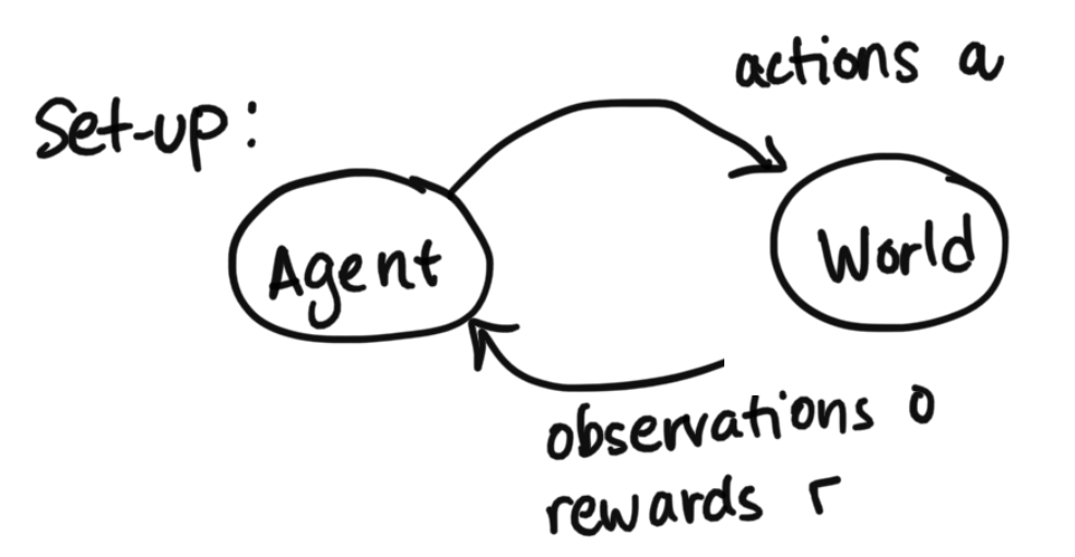
Some Notation, Definitions, and the Goal
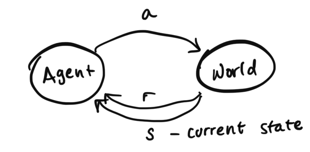
To explain the setup diagram above, the agent can send actions to the world, and the world will return observations that we call $o$ and rewards that we call $r$.$o$ represents observations
$r$ represents rewards
$t$ represents the time stamp
$\gamma$ is our discount factor which is between [0, 1) (in the future, rewards are worth less by a factor of $\gamma$ per round of time)
With the above information, we have:
$E [\sum_t \gamma^t r_t]$ represents expected sum of discounted rewards
Goal: agent should choose the actions to maximize the expected sum of discounted rewards.
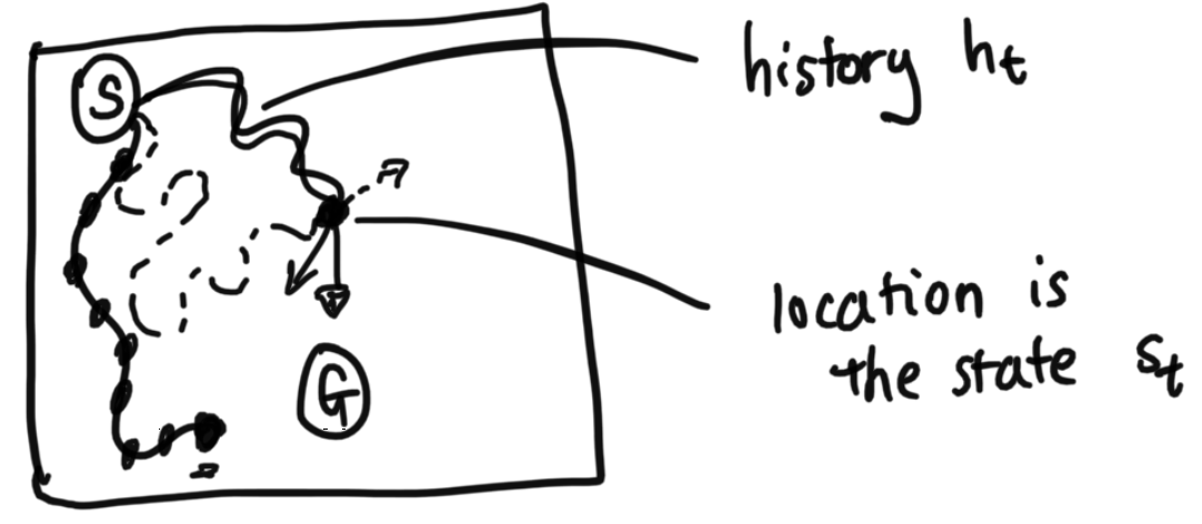
$h_t = \{a_0, o_0 r_0, a_1, o_1, r_1 ... a_t, o_t, r_t\}$ represents the history of actions, obsevations, and rewards from time 1 to our current time t
State: summarizes a history such that making predictions about the future given the state is equivalent to making those same predictions given the entire history.
Breaking Down Definition of State
Let's say instead of a person that this was a car instead, however, and that the car's velocity matters. If the car was coming in at 100 miles per hour from the left, moving "Down" would require a huge turn, versus if the car was driving in slowly from above, at 10 miles per hour, the action "Down" would cause the car to move differently in each scenario. This means that only knowing the car's location is not enough to define the car's state. We would want to incoporate in the velocity, the acceleration, and essentialy everything we need to be able to predict what happens next. State is all information needed to be able to ignore the past. If all of this information is available to us, then we say the system is Markov in state.
Note: this is the official definition of state. Some papers in the literature will sometimes use approximations of states. Say, for example, you might choose to use a single frame (a still snapshot) of a video game (such as Super Mario Bros) as a state. Therefore from the still frame, you can see where each object (such as Mario, bricks, and evil mushrooms) is located on the screen. But to really predict how the objects move, you actually need the velocity of the objects (is Mario running? in what direction are the mushrooms walking?) to predict what happens next and to be able to call the system Markov. It's possible that the paper will just say, "We will choose to use just the frame as our approxmiation of state". It's just important to note that that is exactly what it is: an approximation of a state. However, the formal definition of state is still everything you need to know to be able to predict what's next. We will use this definition for state for the next 3 lectures.
Tying Back and Fully Defining our Markov Decision Process
Now let's fully define everything:
This system can be described using this tuple of information: $$\{S, A, R(s, a, s'), T(s' | s, a), \gamma, p_0\}$$ $S$ are all possible states
$A$ are all possible actions
$R(s, a, s')$ is the reward for doing action $a$ in starting state $s$ and landing in state $s'$
$T(s' | s, a)$ is a matrix of transition probabilities, which describe $p(s' | s, a)$, the probability of landing in state $s'$ from taking action $a$ from starting state $s$. Notice this is a similar idea to the last time when we were defined T(s'|s) for Hidden Markov Models. The only difference is that here, transition probabilities depend on the action.
$\gamma$ is the discount factor. $p_0$ is some starting state.
Goal: Find the best policy. We use $\pi$ to denote a policy. Policies can be stochastic, or describe a distribution over actions ($\pi(s, a) = P(a|s)$), or determinstic and be equal to 1 action ($\pi(s)=a$). Stoachastic policies have a probability distribution across actions for a given state (what probability to play each action with). Deterministic policies we simply have one predetermiend action in the policy to play for each given state. These both are commonly used notations.
The best policy is as follows: $$max_\pi E_{T, p_0} [\sum_t \gamma^t r_t]$$ Here, $T$ and $p_0$ represent transition probabilities and the initial starting state of the world. The agent does not have control over the world. The agent does control its own actions. We are trying to determine the best actions for the agent to take: the actions that maximize the agent's returns that it gets in the world.
How to Solve using Policy Iteration (Method 1)
Over the this lecture and next, we will cover three methods of sovling an MDP. Each will have their pros and cons. There's a lot of literature on this topic that includes more complex methods, but overall the three we cover are intuitive and scale relatively well. Additionally, the complex methods build off these simpler methods here, so this is laying down important groundwork.First, let's explore policy iteration. At a high level, policy iteration iteratively evaluates a proposed policy, and then performs policy improvement.
Policy Evaluation
To understand policy iteration, we first much understand policy evaluation. Policy evaluation is used to estimate the expected reward at each state given a particular policy $\pi$ to follow at each state. More formally, given a $\pi$, policy evaluation calculates $E[\sum \gamma^t r_t]$. Let's start with some definitions...Define $V^\pi(s) = E_{\pi, T}[\sum \gamma^t r_t]$
Here, the notation $V^\pi(s)$ represents the ``value'' of policy $\pi$. We define the value as the expected sum of discounted rewards the agent will receive. Note: the $\pi$ is in the expecation just in case it's a stochastic policy. If $\pi$ was deterministic, we wouldn't need to do this.
Define $Q^\pi(s, a) = E_{\pi, T} [\sum \gamma^t r_t | s_0=s, a_0=a]$
Here, we define this Q as a slight altercation of the above V. You can think of $Q^\pi(s, a)$ as experimenting with a policy. We're essentially saying: For one instance of time, take action $a$ which lands us in some $s'$ instead of following policy $\pi$. Then for each following time step, the agent will follow the policy $\pi$ the rest of the way. This is the definition of $Q^\pi(s, a)$, which will be used later.
From this point onwards, let's have our rewards $R(s, a)$ be deterministic. Remember that the randomness in $R$ comes from the transition probabilties, which can make the rewards different. Note: this is a very reasonable restriciton, because we can always redefine $R(s, a) = E_R[R(s, a)]$. Since this whole R term will be taken over expectation anyways, if we just redefined R to be deterministic, we would be fine.
From this point onwards, let's also have our $\pi$ be a deterministic pi(s). This is a reasonable restriction, because for MDPs, it turns out there will always be a determistic optimal policy for a MDP. The proof for this claim is outside the scope of this class, but the general idea is that there is always going to be a determistinic strategy that will exploit the highest possible discounted reward.
Note: this assumption does not hold in a multiplayer game. Imagine rock paper scissors: with two players, the optimal $\pi$ has to have some randomesnss, because if you always played scissors the opponent could always play rock and beat you consistently.
Bellman Equation: $$V^\pi(s) = R(s, \pi(s)) + \gamma \sum_s' T(s'|s, \pi(s)) V^\pi(s')$$ Here we introduce the Bellman Equation. In our below derivation, we will show that the Bellman Equation is recursive with respect to each time step $t$. Notice that because we assumed policy $\pi$ is deterministic, $\pi$ is a function of only $s$ instead of both $s$ and $a$.
How did we derive this Bellman equation? Let's start from our definition of $V^\pi(s)$: $$V^\pi(s) = E[\sum_{t=0} \gamma^t r_t | s_0 = s]$$ $$V^\pi(s) = E[R(s_0, \pi(s_0)) + \sum_{t=1} \gamma^t r_t]$$ We can extract out the first time step. $$V^\pi(s) = R(s_0, \pi(s_0)) + E[\sum_{t=1} \gamma^t r_t]$$ We can pull out a factor gamma to help us start to recreate V but for s'. $$V^\pi(s) = R(s_0, \pi(s_0)) + \gamma E[\sum_{t=1}\gamma^t r_t | s_0 = s_1]$$ Note that $s_1$ is unknown. It depends on where taking $\pi(s)$ after $s_1$ lands us. $$V^\pi(s) = R(s_t, \pi(s_0)) + \gamma E_{s_1 | s_0} [ E [ \sum \gamma^t r_t]]$$ Since the state space is discrete, we can use summations to rewrite the expectation. $$V^\pi(s) = R(s_0, \pi(s_0)) + \gamma \sum_{s_1} T(s_1 | s, a) E_{T, \pi}[\sum \gamma^t r_t | s_0' = s_1]$$ The right part of this equation is now a redefinition of $V^\pi(s')$ so we have completed our recursion for 1 time step. $$V^\pi(s) = R(s, \pi(s)) + \gamma \sum T(s' | s, a) V^\pi(s')$$ The idea here is that the value of being in a particular state is equal to the immediate reward that the agent gets from following policy, plus a discounted expectation of what the future value is at the next time step.
So how do we actually solve this to complete Policy Evaluation?
So far we've just written out a Bellman equation, and justified why it's correct mathematically and conceptually. But we still haven't solved for $V^\pi(s)$ yet.
The good news is, if the state spaces and actions spaces are discrete, it is easy to solve for $V^\pi$! First, we note that the Bellman equation is a linear equation. Across a set of $|S|$ states, we have $s$ unknowns and $s$ equations, with one Bellman Equation for each state. This means we can simply solve the system of equations.
Method 1: Solving for V
Write down our system of equations in vector form: $$V^\pi = R^\pi + \gamma T^\pi V^\pi$$ $V^\pi$ is a vector. $R^\pi$ is a vector, where each element is $E_\pi[R(s_t, \pi(s_t))]$ if R is random, or $R(s_0, \pi(s_0))$ if R is deterministic. $T^\pi(s'|s)$ is $T(s'|s, \pi(s))$.When we solve the system of equations, we get closed-form solution: $$V^\pi = (I - \pi T^n)^{-1} R^\pi$$
Method 2: Solving for V
We can also solve for $V$ iteratively, updating our estimates for $V^\pi$ until they converge. This method is used more in practice, as this method tends to be more stable. First, initialize $\hat{V}^{\pi(s)}_{k=0}$ to be whatever constant you'd like.Define $\hat{V}^{\pi(s)}_k$ as:
$$\hat{V}^{\pi(s)}_k = R(s, \pi(s)) + \gamma \sum_s' T(s' | s, \pi(s))V^{\pi(s')}_{k-1}$$ The $V^{\pi(s')}_{k-1}$ represent our old estimate of $V^{\pi(s')}$ at iteration $(k - 1)$ of the algorithm. We can use this old estimate at iteration $(k - 1)$ to compute a new estimate at iteration $k$. The intuition is that with every iteration, we will push our our old estimate into the discounted future. $$\hat{V}^{\pi(s)}_k = R(s, \pi(s)) + \gamma \sum_s' T(s' | s, \pi(s)) [R(s', \pi(s')) + \gamma \sum_s'' T(s'' | s', \pi(s'))V^{\pi(s'')}_{k-2}]$$ Therefore the originally initialized $\hat{V}^{\pi(s)}_{k=0}$ is ``pushed out'' into the future. If we expand the math out, we end up with term $\gamma^2 \hat{V}^\pi_{k=2}(s'')$, where we notice for each iteration, we multiply this term by another $\gamma$. Essentially, we have $\gamma^\textrm{iters} V_0^\pi$.
This is a contraction because $\gamma$ is less than 1 (by definition for us), and eventually this pushes our wrongly initalized value matrix $\hat{V}^{\pi(s)}_{k=0}$ so far into the future that it doesn't matter anymore.
Tying Back to Policy Iteration
Now we have two ways to perform policy evaluation, or solve for $V^\pi(s)$. Now, let's return to our goal of policy iteration. As you can see, in it, we use policy evaluation. The algorithm is given below: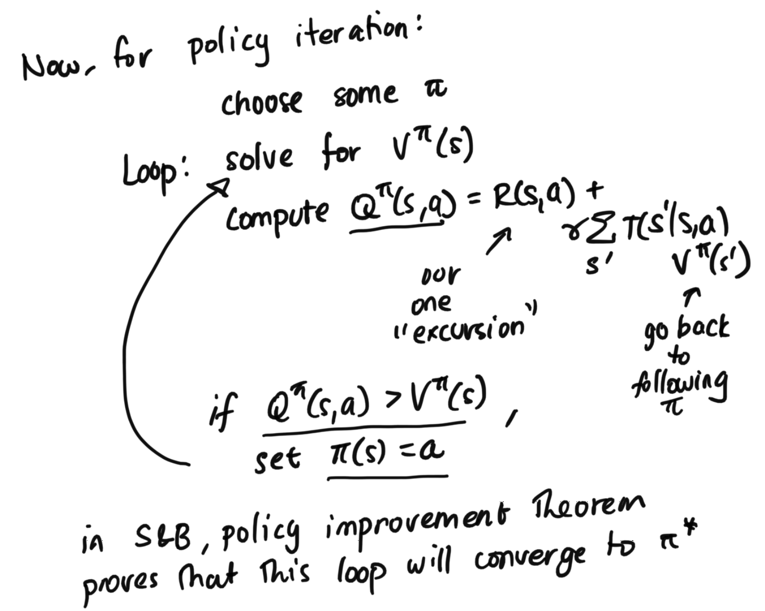
Overall, at a high level, you can think of like this: we started with a policy, we tried some excursions, evaluated them, then improved our policy. We then repeated this, iterating until our policy was optimal.