Date: April 13, 2020 (Lecture Video, iPad Notes, Concept Check, Class Responses, Solutions)

Relevant Textbook Sections: 10

Lecture 19 Summary

• Intro: Time Series
• Setting up our Hidden Markov Model
• Questions We'd Like To Answer
• Solving Questions in Collection 1
• Solving Questions in Collection 2

Intro: Time Series

Today, we will be covering time series. To contextualize this a bit, remember in our last two lectures we were covering graphical models. Graphical models, as a reminder, can be applied to anything on the probablistic side of the cube, whether supervised or unsupervised, whether continuous or discrete. They allow us to add structure onto an existing problem or situation, making it easier to solve and reason with. Today, we're basically going over a specific structure of a graphical model. We will be looking at time series.

Before we move on, let's consider a few real world examples of time series. One of Finale's former PhD students, Joe Futoma, looked at time series' in the context of chronic kidney disease. Specifically, he and his team worked on predicting disease progression over time. This was critical, as those who are identified to be more at risk to moving towards a later stage of the kidney disease sooner need earlier treatments from doctors.

Another real world example is Google looking at trends in the flu using Google Search data. Normally, it takes a long time for CDC to actually get flu data (since the patient has to get sick first, go to the doctor, the doctor has to aggregate the data, the data has to get sent to the CDC and get reviewed). So to speed up the process, Google used search data to predict the real time amount of flu in the population (beacuse people search symptoms when they get sick). The predictions actually were matching with the CDC data really well for a long time, up till the December of 2012, when the Google data predicted rates that were way too high. This is a good lesson for us to examine. On the one hand, this was a very clever use of data to inform the CDC about flu rates in real time, but it also teaches us how important assumptions are when we make predictions. We are dealing with lots of non-stationary variables in our time series models, where people might change their search behaviors, or some events might lead to specific spikes in flu symptom searches. Hence, the execution of our modeling is super important. We need to constantly watch for alignment as we deal with forecasting models, making sure we monitor and validate our models over time.

Setting up our Hidden Markov Model

Let us set up our hidden markov model below.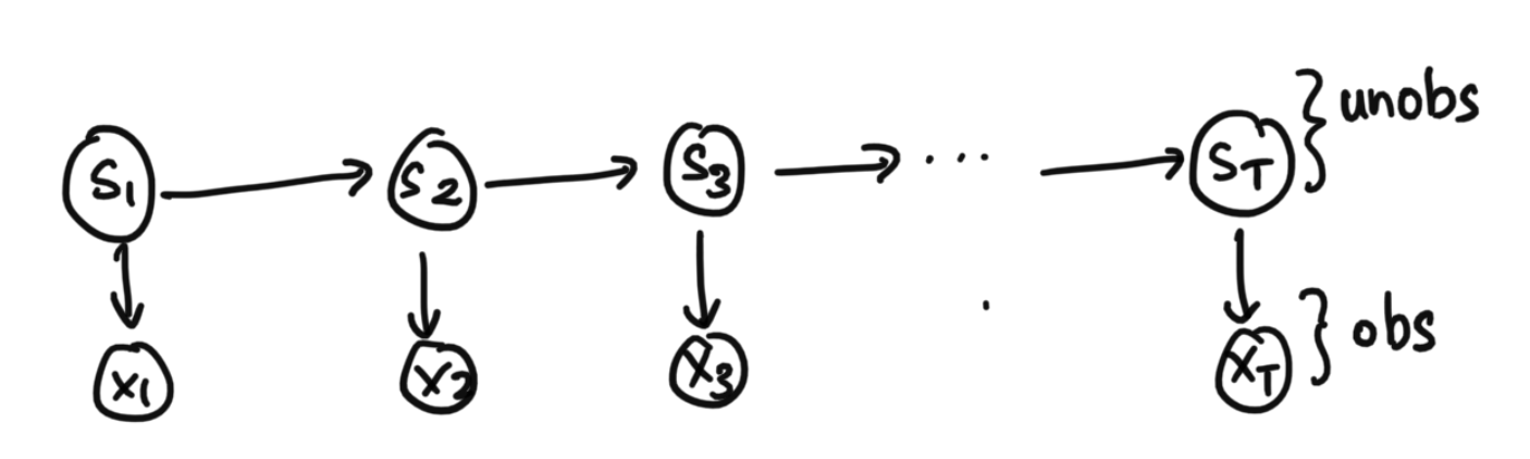 Note: We're changing the notation from z to s because s refers to state and the more commonly used term in this literature just by convention.

The states above are unobserved. The x's are the obersvations. As an example, the s states might be true disease states of the patient over time, and the x observations could be the patients biometrics, such as their temperature or some other measure. In another example: the states could be words being said, and the observations could be the actual audio signals recorded by microphone. A final example: the states could be the locations of a given object, and the observations could be the geolocation data given from our senors. As you can see, this form of graphical model comes up a lot in real life.

Three Main Global Unknowns/Parameters

In our graphical model above, we have three main global unknowns or parameters. Specifically, they are:

1. $p_0(s)$: The prior. Which state do we start in? To get our first time step t=1, we have a prior at 0 which has a probability break down of what state we'll be in at t=1.
2. $T(s' | s)$: The transition probabilities. This is also known as $p(s'|s)$, as it's the probability of arriving at s' given we are coming from state s.
3. $\Omega(x | s)$: The observation probablities given states. This is also known as $p(x | s)$, the probability that we see what we see in the observation for a given state.

Local Unknowns

We also have local unknowns:

$s_1, s_2 ... s_T$ for every sequence $x_1, x_2 ... x_T$

Note that we're using subscript for time index. We will use uppercase T to denote the end of time, as in the last time step. We will use lowercase t to denote some arbitrary point in time.

Questions We'd Like To Answer

Collection 1: Given Globals, Solve for Locals

Overall, given $p_0$, $T$, and $\Omega$, we want to be able to find out things about s and x.

1. Filtering: $p(s_t|x_1 ... x_t)$. What is the level of flu right now, so that we can allcoate the right amount of resources (useful for real-time monitoring
2. Smoothing: $p(s_t | x_1, ... x_T)$. After COVID-19 is over, after we have all the observation data till the end time at time step capital T, what were the true number of cases at any point in time (given all the data available)? Here, we're looking back in time after the fact.
3. Probability of Sequence: $p(x1 ... x_T)$. Perhaps we want to detect outliers in audio, to detect whether a sequence of noise was simply just background noise or an echo. We can use the probability of the sequence as a way to tell if it is an outlier or not.
4. Best Path: $argmax_s p(s_1 ... s_T|x_1 ... x_T)$ What's the most likely overall trajectory?
5. Prediction: $p(x_t | x_1 ... x_{t-1})$. Perhaps we want to predict the obersvation itself, not the state. Example: we may want to predict the hopstial utilization rate tomorrow given what has happened so far so we can better plan for this and allocate resources properly (as opposed to predicting the actual disease itself, which are the states in this case).

Collection 2: Given x's, Solve for Globals

We also want to learn the globals given the x's. Specifically:

Given ${(x_1 ... x_T)}$, find the ML or MAP of $p_0$, $T$, $\Omega$

This is important because we need to learn the globals before we are able to do the collection of problems in collection 1.

Solving Questions in Collection 1

As a recap, collection 1 refers to solving the problems listed from before when $p_0$, $T$, $\Omega$ are known.

Forward-Backward Algorithm

In order to solve the questions in Collection 1, we are going to use the forward-backward algorithm from last class. Remember that we already went through the algoirthm last class for how to get the optimal order of variable elimination for polytrees. Our time series set up here is indeed a polytree, as we also mentioned in last class in our brief example. The Forward-Backward algorith is essentially a specific instantiation of the same algorithm from last class for the time series case. You can think of this either as a review of last class to make sure we really get it, or as a deepr dive into a particular useful scenario.

Diagram Depicting Forward and Backward Messages

As we go through the algorithm, we notice some interesting properties about the math we do. Specifically, at a conceptual level, we'll see later how we esesntially have these $\alpha$ terms taht are "messages" that feed information forward, and these $\beta$ terms that are "messages" that feed information backward (hence the name). See the diagram below for details.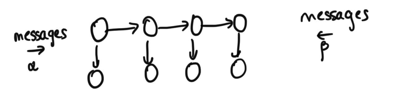

A Dive Into the Math

Let's now dive into the math. Let's start with discrete state to keep things simple.

First, we're going to have $p_0(s)$ which is going to be a vector of size |S| elements.

Looking at $p(x_1)$

Let's first look for $p(x_1)$ and break down the math. $$p(x_1) = \sum_{s_1} p(s_1) p(x_1|s_1)$$ Here, $p(s_1)$ is $p_0$, an |S| dimensional vector, since $s_1$ is the first state in the sequence (and the prior $p_0$ tells us what our $s_1$ will be via it's vector of probabilities). $p(x_1 | s_1)$ is our $\Omega(x_1 | \cdot)$, the probabilities of $x_1$ being the way it is given $s_1$.

How did we arrive at this equation? Remember our equation from last time. From before, we know that first we can prune out a bunch of variables. All we need to consider are the ancestors of our query and evidence variables, and here that means we only consider $s_1$ as it's the only acnestor of our query (and we have no evidence variables). So, hence, then we sum out $s_1$ to arrive at our answer. This is important to note: it is definitely interesting that we don't need to consider $x_2$, $s_2$, and everything onwards in the future that we also haven't observed yet.

Looking at $p(x_2 | x_1)$

First, we know that $p(x_2 | x_1) \propto p(x_2, x_1)$. Also, as before, we only incorporate ancestors, which here, are $s_1$ and $s_2$. Let's calculate: $p(x_2, x_1)$, as we can always normalize after. $$p(x_2, x_1) = \sum_{s_1} \sum_{s_2} p(x_2 | s_2) p(s_2 | s_1) p(x_1 | s_1) p_0(s_1)$$ We're going to reorder summations using what we learned in last class. $$\sum_{s_2} p(x_2 | s_2) \sum_{s_1} p(s_2 | s_1) p(x_1 | s_1) p_0(s_1)$$ When we consider the $\sum_{s_1} p(s_2 | s_1) p(x_1 | s_1) p_0(s_1)$ portion of the equation, we can think of this as message $s_1$ shares with $s_2$ about likely $s_2$ is to be certain things given this info. Officially, this term is equivalent to $p(s_2, s_1)$, so we're basically incorpating in information from $s_2$ with $x_1$. To give a bit more detail, $p(s_2 | s_1)$ is going to rely on T, our transition matrix. $p(x_1 | s_1)$ is going to come from our $\Omega(x_1 | \cdot)$, similar to how we did it in the previous problem. $p_0$ is the prior, as before as well.

On the other hand, the other part of the computation is $\sum_{s_2} p(x_2 | s_2)$, which is representing how we incorporate in our other information, which we have from $s_2$. Concretely, $p(x_2 | s_2)$ is going to come from our $\Omega$.

Doing these two parts together glues togehter these two pieces of information together, resulting in our joint $p(x_2, x_1)$.

Extending this Method to Arbitrary t

Let's extend the above method to arbitrary time step t. To do this, we will formally define our $\alpha$'s and $\beta$'s, which are the same ones from the diagram from before, and which relate closely to the math we just did above in those specific examples.

Defining Alpha

First, $\alpha_t$ is essentially $p(s_t, x_1...x_t)$, in terms of what it captures from the graphical model. Below, we actually break down the math. Below is first our base case using the prior, then the general case:

$\alpha_1$ = $p_0 \odot \Omega(x_1 | dot)$

$\alpha_t = [\sum_{s'} \alpha_{t-1}(s') T(s|s')][\Omega(x_t | s)]$

Note: this is a size |S| vector. The above equation shows how to calculate the value of one state, but really this needs to be done for each possible state and then combined into a size |S| vector. This is the same logic as applied in the math in the above equations if you want to refer to concrete examples.

To explain the intuition of the math, with regards to the left term, $[\sum_{s'} \alpha_{t-1}(s') T(s|s')]$, we're essentially getting the previous alpha, $\alpha_{t-1}(s')$, applying the transition to get to the current state. This corresponds prefectly to our specific example from before, where with $\alpha$, we're incorporating information from the past.

Then, the other term that's part of $\alpha$ is $[\Omega(x_t | s)]$, which incorporates information about our current observation. Again, this is the same as in our specific example above.

Defining Beta

$\beta_t$ is a very similar idea to $\alpha$ but about the future. It is essentially $p(s_t, x_{t+1} ... x_T)$, in terms of what it captures from the graphical model. In words, this means if I see the future, I want the joint distribution of the future and the current (rather than the past and the current). Below, we actually break down the math.

$\beta_T(s) = 1$ (no information at initialization)

$\beta_t(s) = \sum_s' \beta_{t+1} (s')p(s'|s)\Omega(x_{t+1} | s')$

$\beta_{t+1}$ is info from future, $p(s' | s)$ is telling us where we might be now, $\Omega(x_{t+1} | s')$ is the next obersvation. Note now we're considering t+1 in the $\Omega$, not t, since we are looking at the future and not the past.

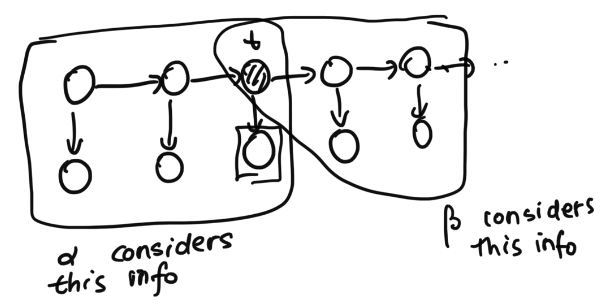
Diagram and Convention

Below is a diagram that maps out the $\alpha$ and the $ \beta$ on the graphical model. Note that the current observation had to put either in alpha or beta, and just by convention it was put with the prior data (this observation has a square drawn around it).

Using $\alpha$ and $\beta$ Is Efficient

So say we wanted to find $p(s_t | x_1 .. x_T)$. Ultimately, all we need to do is: $$p(s_t | x_1 .. x_T), \propto \alpha_t(s) \beta_t(s)$$ The beauty is that this can be efficiently computed. This is polynomial and has no exponential blow up with respect to the length of the time series.

Note: $\alpha$ and $\beta$ can let us compute lots of other things, including helping us find most likely paths and more. Due to time constraints in CS181, these won't all be covered.

Solving Questions in Collection 2

Next, briefly, we consider how to find $p_0$, $T$, $\Omega$.

First, we note that if we had s, then solving maximum likelihood of $p_0$, $T$, $\Omega$ would be easy. We would just get the empircal dsitribution over $s_0$'s to get $p_0$. For each s, we could count how often an s' happens to get the transition matrix. Essentially, we can collect everything by just gathering the data.

In addition, the process from above tells us how forward-backward algorithm allows us to get s given the globals.

Combining these two ideas, we see that we apply block coordinate ascent (the same thing we've gone over many times over the last few weeks) to solve!