Date: March 2, 2020 (Concept Discussion and Possible Answers)
Relevant Textbook Sections: 5.1-5.3
Cube: Supervised, Discrete, Nonprobabilistic
Lecture 10 Summary
- Intro: Real World Example of SVMs
- Intro to Max Margin (a new objective function)
- Hard Margin SVM
- Soft Margin SVM
- Review of All Loss Functions
Relevant Videos
Intro: Real World Example of SVMs
Until recently, Support Vector Machines were the workhorse of machine learning. They were used in all kinds of contexts. One quick example is if you wanted to classify different types of cells, you could use an SVM to sort cells into different types. This worked really well. Another example in Boston is the Casella plant which sorts trash and recycling. Cambridge and our surrounding areas have single stream recycling, and we just dump all recyclable things into a bin. How do they separate it back out? Some of it is manual, as you have to take big things out with your hands (for example, some people put bikes in the recycling for some reason). Magnets are used to get certains metals, but for plastics, there's no easy mechanical way of separating different types of plastics. Because of this, a long time ago when we recycled plastic, we had to use the numbers on the plastic to figure out which bin to throw our recycling into. Now, you don't have to do this, as SVMs come into play! There is a conveyer belt takes a picture of the plastics that move through and using SVMs, we can tell what type of plastic a given item is and automatically send it down the right path. Note: while SVMs can techincally be used in regression, SVMs are mostly used in classification problems.Max Margin (a new objective function)
Before we dive into SVMs, we have to dive into what max margin is first. What is max margin's relationship to the SVM? The max margin is an objective function that is used in SVMs. Note: because it is an objective function, the max margin can also be used in other techniques, and there is actually a whole family of techniques called margin methods. So far in the past, our objective functions have included negative log likelihood, squared loss, 0/1 loss, hinge loss, log loss, etc. We've really done nothing too special or fancy. While this was okay for regression generally speaking, it wasn't as good for classification. In classification, to put things into full context, we wanted to start with a 0/1 loss, but we realized this was too difficult to optimize, so we created proxies (all the other loss functions we used in classification). Now, we are going to look at the max margin objective.Some Motivation on why we want Max Margin and what it is
Let us draw the following picture: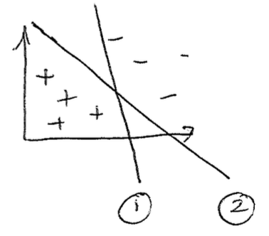
Which boundary would you prefer, 1, or 2? The class voted overwhelmingly for boundary 2. Which boundary would the perceptron prefer? It would find both boundaries to be the same! That's exactly the issue we are trying to tackle, we want a loss function that will try to give us line 2. How do we formalize the reasons we like line 2? Loosely speaking, we're trying to balance out the empty space between the two classes...
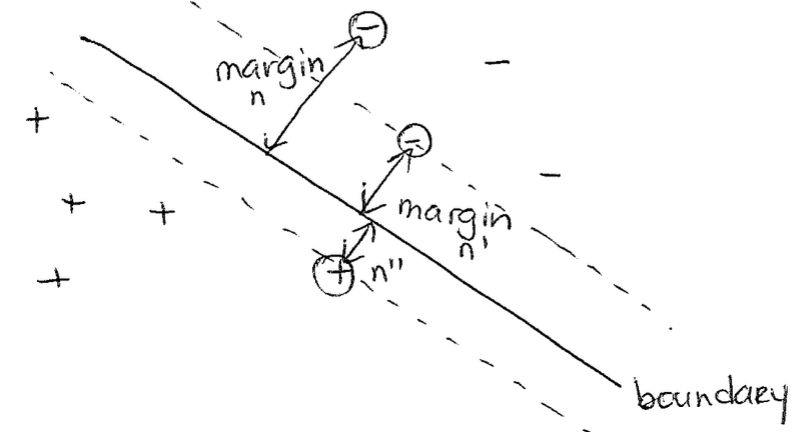
First, let us define the distance between a given point $x_n$ and the boundary, and call this the "margin" of $x_n$. Essentially, we are going to try to put the put the boundary in the middle by maximizing the "min margin" (which is why this is called max margin), as in put the boundary as far away as possible from the closest point (the min margin) to the boundary. This will in theory lead to the lowest generalization error. This idea is depicted below.
Hard Margin SVM
First, to keep things simple, let's look at a binary classification setting, where $\hat{y}$ is 1 or 0. In addition, we're going to focus on the linear case today: $f(x, w) = w^Tx + w_0$ (next class we'll look at the nonlinear case). These previous two sentences refer to general properties we're choosing to keep things simple in our SVM example.In addition, we're going to assume that the data is separable, which is what makes this a "hard margin" formulation. This isn't required (and also may seem unrealistic for real world data), but makes the initial math set up much easier, and makes it easier for us to later extend this idea to other versionns of SVM. The hard margin SVM will force all the points to be classified correctly (since it is separatable). If you gave non-separatable data to a hard margin SVM it would just say no solution.
Writing out the Objective of our Hard Margin SVM using Geometric Intuition to Help
At a high level here, what we want to do in this section is to define formally the margin so that we can actually maximize the min margin.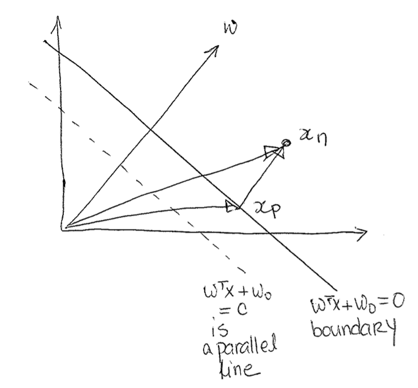
Next, we see that $x_n - x_p$ is parallel to w, since we know that w is orthogonal to the boundary, and we specifically decomposed $x_n$ in a way that $x_p$ to $x_n$ is also orthogonal to the boundary. Because of this, we can write it as $r \frac{w}{||w||_2}$ where r is the margin and $\frac{w}{||w||_2}$ is the unit vector in the direction of w.
Now we can rewrite all of this as the following: $$x_n = x_p + r \frac{w}{||w||_2}$$ Next, we multiply this all by $w^T$. $$w^Tx_n = w^Tx_p + r \frac{w^T w}{||w||_2}$$ Now we add w_0 to both sides. $$w^Tx_n + w_0 = w^Tx_p + w_0 + r \frac{w^T w}{||w||_2}$$ Remember that $w^Tx_p + w_0$ by definition is 0 since $x_p$ is on the boundary and anything on the boundary is defined to be 0. $$w^Tx_n + w_0 = r \frac{w^T w}{||w||_2}$$ We can simplify because we know: $\frac{w^T w}{||w||_2} = \frac{||w||^2_2}{||w||_2} = ||w||_2$
This means now we have:
$$r = \frac{w^Tx_n + w_0}{||w||_2}$$ This above is the signed distance. We can multiply by $y_n$ to get the unsigned distance, which is exactly the margin (this works if everything is correct, as the effect of multiplying by $y_n$ always makes the result positive). This is good, because we now have the margin, so we can actually maximize the min margin.
The equation below is saying given one data point, what is the margin. $$\textrm{margin}(x_n | w, w_o) = y_n(\frac{w^Tx_n + w_0}{||w||_2})$$ Note on terminology in the equation above. If we remove the normalization factor $||w||_2$, and we look at just the $y_n(w^Tx_n + w_0)$ term, this is known as the functional margin.
We want the minimium margin across all the data though, and then we want to maximize that whole term. Let's first write out the minimum margin across the data. $$\textrm{margin}({x_1, x_2, ... x_n} | w, w_o) = min_{x_n} y_n(\frac{w^Tx_n + w_0}{||w||_2})$$ Now, finally we maximize the whole thing.
$$max_{w, w_0} min_{x_n} \frac{1}{||w||_2} y_n (w^Tx_n + w_0)$$ This computation will turn out to be nice.
Deal with Overparamaterization and Simplify Objective
We notice that what we have above is overparamaterized. What that means is there are too many parameters for us to choose, and not in a way where these paramaters have meaning, but in the sense that the extra parameters are meaningless. What exactly does that mean?As an example, note that for: $w^T$ and $w_0$, we could also substitute in instead, a new $w = \beta w$ and a $w_o = \beta w_0$, as in basically we scale the parameters with a scaling factor $\beta$ that we choose. It turns out, no matter how much we scale it, it doesn't actually matter how long w is. Any scaled w will work, as they're all perpindicular to the same boundary, which will lead to all the same results. So this is where the Overparamaterization comes from.
To help get rid of this overparamaterization situation, let's just pick our own scaling factor. Specifically, let's pick a scaling factor such that $y_n(w^Tx_n + w_0) \geq 1$. This helps in the following way: $$max_{w, w_0} min_n \frac{1}{||w||_2} y_n (w^Tx_n + w_0)$$ We can pull out the term that doesn't depend on n. $$max_{w, w_0} \frac{1}{||w||_2} min_n y_n (w^Tx_n + w_0)$$ Now let's add in our constraint. $$max_{w, w_0} \frac{1}{||w||_2} min_n y_n (w^Tx_n + w_0) \textrm{ s.t. } y_n (w^Tx_n + w_0) \geq 1$$ Here, we pause for intuition. We know from before that we can scale the w's, and the results are really the same. In our problem we want w to be small because we are trying to maximize 1/w, and also minimize $w^Tx + w_0$. This mean's we would really just keep trying to make w smaller, that is, until we hit the new constraint we just set (and this is why we set it). Because of our set up, we also know that this whole term, $min_n y_n (w^Tx_n + w_0) \textrm{ s.t. } y_n (w^Tx_n + w_0) \geq 1$, is going to go to 1, as w keeps getting scaled smaller until we hit the constraint. We can prove this quickly in our heads because if it's not yet at the cosntriant, we aan always continue to scale w to be smaller until we hit the constraint. So now we have: $$max_{w, w_0} \frac{1}{||w||_2} \textrm{ s.t. } y_n (w^Tx_n + w_0) \geq 1$$ Let's change this now to: $$min_{w, w_0} ||w||_2 \textrm{ s.t. } y_n (w^Tx_n + w_0) \geq 1$$
Optimization Trick
Minimizing $||w||_2$ with respect to $w$ and $w_0$ is the same is miniziming $w^Tw$ with respect to $w$ and $w_0$, as squaring it doesnt change where the minimum is. So now we're looking minimizing the length squared. This is really cool beacuse now we have a quadratic program with linear constraints; this is a convex problem which has a lot of excellent solvers out there: cvxopt, cvxpy, sklearn (we do not want to code these ourselves, we can leverage the work of others)!Soft Margin SVM
What if the data is not separable and we still want a solution? We can have a relaxed soft margin formulation. For any particular point, we can define how badly it is from the margin using slack variables.We define the slack variable to be $\xi_n$ for the n'th data point. $\xi_n$ will be 0 if a point is correct and also out of the margin violation. Otherwise, $\xi_n$ will be the distance from the margin. The idea behind this is kind of like hinge loss, where we linearly increase as a point is more and more wrong.
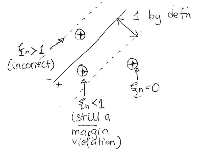
Now, our new formulation in the equations sense will be: $$min_{w, w_0} \frac{1}{||w||^2_2} + C \sum(slack)_n$$ Such that... $$y_n(w^Tx_n + w_0) >= 1 - \xi_n$$ $$\xi_n \geq 0$$ To give some intuition on this, essentially we are "pretending" that the margin is 1 and writing our constraint in that same way, but allowing for some slack, for some miscliasfied points.
If we make C really big, we will be enforcing the constraints more. How do we set the C though? We would want to find this using cross validation (although sklearn finds it for you automatically). Also, it turns out also that this is still convex, so we can still use solvers! We have converge guarantees!
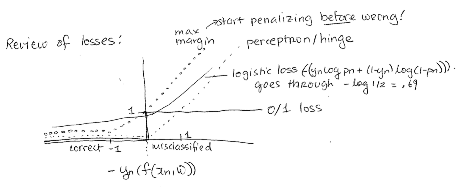
Review of All Loss Functions
Below is a graph of a bunch of loss functions we've seen. The intuition behind the new max margin loss we just learned today is that it starts penalizing you before you're wrong, as in it even penalizes you when you're correct. This helps you avoid future mistakes.