Date: April 20, 2020 (Lecture Video, iPad Notes, Concept Check, Class Responses, Solutions)
Lecture 21 Summary
- Intro: Real World Thinking on Designing the Reward Function
- Quick Recap of MDPs from Last Time
- Planning using Value Iteration (Method 2)
- Planning using Linear Programming (Method 3)
- Planning Using Forward Search (Method 4)
- Reinforcement Learning
Intro: Real World Thinking on Designing the Reward Function
In today's lecture, we will first wrap up MDPs from last time, then cover reinforcement learning. As usual, we begin with a real life example that relates to what we've been covering these past lectures.Last class, we ended with a concept check that investigated how changing the reward function affects the optimal policy (if we shift the rewards, or scale the rewards, we found that thankfully we still get the same optimal policy, which is good in the sense of robustness: logically, scaling or shifting the rewards indeed shouldn't change the policy). However, overall, specifying a reward function in real life is actually pretty hard. One thing that's important to note is, our techniques for solving these MDP and RL problems is getting better and better. But one of the harder problems is actually set up, and a particular challenge is: how do you specify a reward function? Unfortunately, because this is complicated as it involves both human factors and machine factors, we won't have time to touch on this in this course. But in today's intro, we dig into some quick examples.
Suppose you were teaching an agent to clean the house (say, a roomba). We might start off by specifying a +1 point for every dirt the roomba picks up, a clear and obvious reward function. Quickly, we realize that as the reward designer, we didn't consider enough details. Let's say you own a pet cat, and the roomba detects some dirt behind the cat. It will drive straight into the cat to try to get the +1 as quickly as possible, and the cat will be very upset. So perhaps as the reward designer, maybe we adjust the reward function, and we say +1 for picking up some dirt, but -1000 if you hit the cat. This will now make the agent go around the sleeping cat, which is good. But what happens next when there's no more dirt left? We've specificed a +1 for each piece of dirt picked up, so the agent might actually start scattering out the dirt again so that it can re-pick it up to maximize it's reward function! This sounds silly, but this is what the agent would do if that was the reward functions. Any agent will simply optimize whatever you've defined. As a result, we must very careful with how we specificy reward functions.
The above example might not be very believable, as we know that our roombas are smarter than that. However, a great example of a challenging reward function to define is one for a self driving car. Let's say you want the agent (the car) to drive safely, and start with a +1 for driving in the lane. If a pedestrian jaywalks though, and right in front of the car, now you can't stay in the lane all the time. What should the car do? We would have to specify this in the reward function. What if there are multiple pedestrians and you're travelling too fast and you must hit at least one of them. Which way should the car veer? Even though we're getting better at solve these MDP and RL problems, we see that designing the reward function can still remain difficult.
For those who are interested, a paper that talks about this topic of reward functions is "Concrete Problems in AI Safety".
Quick Recap of MDPs from Last Time
As a refresher from last time, our MDPs are defined by: $$\{S, A, R(s, a), T(s' | s, a), \gamma\}$$ And our goal is to find the $\pi(s)$ that maximizes $E[\sum_{t=0} \gamma^t r_t]$, expected sum of discounted rewards.Specifically, last time, we covered how to solve the planning problem using Policy Iteration, which we called method 1. See the last lecture's notes for details on that. Today we're going over a couple more methods of solving the planning problem (and don't forget that there are many more out there than what we're covering in CS181).
Planning using Value Iteration (Method 2)
As a refresher, the term planning refers to the problem when we have T and R available (the MDP setting). If we didn't have access to the T and R and had to learn or infer those through actual interaction with the world, then we would be in the reinforcement learning setting instead (more details on the difference between planning and reinforcement learning will come later in this recap).Value Iteration Algorithm
The image below shows the whole algorithm.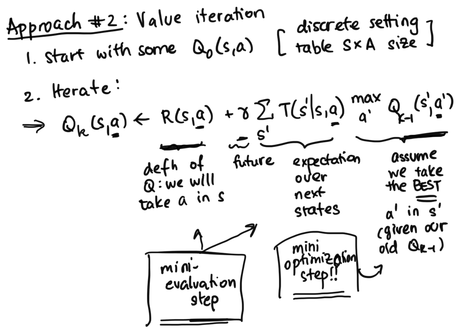
Notes Regarding Value Iteration
- At convergence, we will get the $Q^*(s, a)$
Afterwards, we can extract what we want. $$\pi^*(s) = argmax_a Q^*(s, a)$$ $$V^*(s) = max Q^*(s, a)$$ As a refresher, remember that $Q^*(s, a) = R(s, a) + \gamma \sum_{s'} T(s' | s, a) Q^*(s', \pi^*(s'))$.
- Value iteration will convergence by similar contraction argument as from last lecture, but we won't cover it today in the interest of time
- $\pi$ might converge before Q
Example: Maybe you have the action set of either left or right. Suppose for a given state, you have Q values: 4 for left, 3 for right, so the optimal move is to go left. Perhaps true Q values are actually 3.5 for left and 2.5 for right, so the values have not converged yet. However, the policy is already to go left, and even as we go through more iterations, getting the values closer to convergence, the policy has already converged.
-
Each iteration is fast, but value iteration takes more iterations than policy iteration.
In value iteration, there are a ton of iterations, but we only have a mini evaluation step and mini-optimization step in each iteartion, wehreas policy iteration does a full policy evaluation each time (even though it has less iterations). Because of these counteracting tradeoffs, which one is faster (value or policy iteration) really depends on the specific situation.
Concrete Toy Example of Policy Iteration vs Value Iteration
To see a concrete toy example of policy iteration versus value iteration, see the lecture video from the 31:00 to 48:00 time stamps. This is best viewed in the video as different parts of the tables are underlined during different steps of the algorithm, so static images are much less effective than video.Planning using Linear Programming (Method 3)
One other way of solving the planning problem is using linear programming. Note: this only works for discrete states and actions. Essentially we minimize in the following way: $$min \sum_s V(s)$$ Such that: $$V(s) \geq R(s,a ) + \gamma \sum_{s'}T(s'|s, a) V(s')$$ Which can be rewritten as: $$V(s) \geq Q(s, a)$$ For all s,a.In the top part, $min \sum_s V(s)$, we have V is a vector size s, and this is basically saying make V as small as possible. However, at the same time, we have our condition that $V(s) \geq R(s,a ) + \gamma \sum_{s'}T(s'|s, a) V(s')$, as in that V is at the very least as good if not better than Q. This means that we'll end up with an optimal solution for V, where it's the best of all the Q, and we'll have this across all states and actions. We won't go into this method in detail, but overall in certain situations, solving for a linear programming is very efficient.
Planning Using Forward Search (Method 4)
A final method we'll cover that solves the planning problem is called the Forward Search method. While inefficient and naive, this method is the base of other more advanced algorithms, such as the Monte Carlo Tree Search algorithm (so you can think of this as an example mainly to get you thinking in a different manner). And even while often inefficient, in some cases, it can be useful.When we start at state s, we can think of all the possible actions we might take. Here, we will note down the reward that we get as we take the action. And then, we can expand this tree, and we can think of all the possible s primes that we can get to. Then, once we get to s', we repeat by expanding out all the possible actions (this time we have a $\gamma$ as we note down the reward for the actions due to discounting). Essentially we keep on expanding this tree and sum the expected rewards. In the diagram below, we can visualize what we're doing.
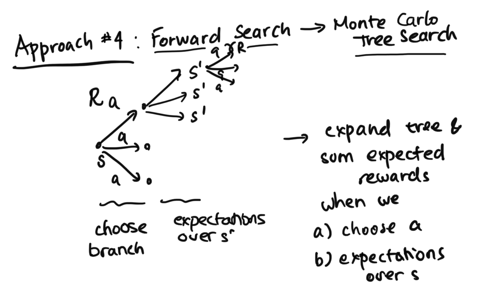
The reason the naive version is super inefficient is because we get this exponentially large tree, so a naive search blows up. However, there are ways of pruning this tree to reduce the amount of work, and there is a whole collection of algorithms that does that, with the most famous of them the Monte Carlo tree search. These algorithms are useful in practice.
As an example, the first initial Go-solvers used Monte Carlo Tree Search, then Alpha Go added a value function so you didn't have to bottom out the whole tree. Alpha Go essentially did a Monte Carlo tree search for a while: thinking about what I might do, what the other player might do, etc. Then they put in a heuristic of board configuration that would tell us if the board looked good for the agent or not, so that they didn't have to do build an infinitely large tree.
Again, remember that the most important things to note are that there are so many methods of solving the planning problem. While policy iteration and value iteration are some of the most common ones, we introduce methods 3 and 4 to give two flavors of other types of algorithms that exist.
Reinforcement Learning
Reinforcement learning is when we're in a situation where we don't have the T and R functions. Instead, our agent can only interact with the world directly, and get the reward given the specific actions that they take. To completely illustrate this, let's look at a real world example.Let's look at the situation where a professor has to figure out the optimal way to get to school for lecture.
In a planning scenario, the professor would a Google Maps app that tells her exactly how long bus X will take, how long walking will take, and how the specific times will vary depending on which roads or turns are taken. This means the model is completely available, and the professor can sit at home, access the model, and plan the best course of action with no risk. All the the professor needs to do is do some calculations ahead of time, find the optimal route, and take the same optimal route every single time.
In the reinforcement learning scenario, the professor doesn't have a map at all. There is no estimate of how long any journey will take, which essentially represents our lack of reward function (since how late we are will tell us how good or bad the situation is: for example, for a professor trying to make lecture on time, being incredibly early is probably fine, being a little early is optimal, and being late at all is very horrible). Since the professor has no information (again remember we have no Google Maps this time), the professor will actually have to try things out. Maybe first, the professor will try walking, and it takes 20 minutes. This seems fine, but should the professor stick with this method the next day too, or should she try the bus? Maybe the bus takes too long, and she'll make it to lecture super late, so that could be risky. But maybe the bus is frequent and only take 10 minutes, leading to a much more optimal journey! We don't have the T and R functions to tell us anything, so the professor has to try things out herself.
Next, let's look at some reinforcement learning algorithms. In CS181, we'll look at three classes of algorithms. Again, note that this is a huge area of study, and that there are tons of algorithms out there which would take entire semesters to cover. We just cover 3 classes here due to time constraints.
Model-Based Learning vs Model-Free Learning
Before we dive into our 3 classes, let us first cover briefly the two broader classes of RL.First, we have model-based learning which is trying to fully estimate the missing world models R and T, and then using a planning (eg. value or policy iteration) to develop the optimal policy after we've found our R and T. In our professor's story example, this would essentially mean to try and create a map, and then using the map to do planning, where the professor can do some calculations at home and then decide how to get to lecture.
On the other hand, in model-free learning, we aren't interested in learning the transition function and reward function. Instead, we hope to directly infer the optimal policy from taking samples in the world. This is like trying the bus out, then trying out walking, etc, in the story from above, and then figuring out what works best just based off those trials.
Within model-free learning, we also see a new challenge of exploration vs exploitation. As we saw in the professor getting to lecture story, we need to ask the question: should we explore new methods (taking the bus) which could potentially work better than what we have tried so far (walking)? Or should we exploit the methods we know already are rewarding (like walking, beacuse even though it takes 20 minutes, we know we'll at least be on time for sure). With these concepts in mind, let us move on to our first class of RL algorithms. We only cover one class today, and cover the other two classes next lecture.
RL Class #1: Value-Based Algorithms
Value-based algorithms lie under the model-free branch of reinforcement learning. For discrete settings, they work in the following way, with these two parts:- Update Q-table (the S by A set of Q values)
- Take an action
Part 1: Q Update Step
Choice #1: SARSA (on-policy)One way to do the update step is the following:
$Q(s,a)$ updated to $Q(s, a) + \alpha_t(R(s, a) + \gamma Q(s', a') - Q(s, a))$
In the SARSA method, we start with old value, $Q(s, a)$. We see that we've involved a $R(s, a) + \gamma Q(s', a')$ term, which represents our new estimate of $Q(s, a)$ given the data. Specifically, $R(s, a)$ represents the current reward, and then we add in a $\gamma$ (to account for a time step) multipled with a $Q(s', a')$ where $Q(s', a')$ represents a single sample from our $T(s' | s, a)$. While this will be noisy in the sense that it's just a single sample, this is our way of approximating the expectation (from when we were doing planning). Essentially, we can think of the whole $R(s, a) + \gamma Q(s', a')$ term as a new estimate of our $Q(s, a)$. Now that we've broken down that down, we can take a step out and look at the bigger picture. Essentially, we start with old $Q(s, a)$, and then our updating it (with a learning rate of $\alpha_t$) by our new estimate of $Q(s, a)$ minus our old $Q(s, a)$. The whole difference term, $R(s, a) + \gamma Q(s', a') - Q(s, a)$, is called the temporal difference (TD) error.
You can see this as a stochastic asynchronous update on this $Q(s, a)$, where essentially, we're taking the old term, and updating it based on the direction of the error. It looks a bit funny, but the idea should still be intuitive. We had some old values sitting around, we looked the error betwen the old value and our new estimate, we incorporated our learning rate, and then we're going to update. The stochastiscity comes from the fact that we are making estimates based off a single simaple at time. With this all in mind, this means that as long as we tune the learning rate properly, since we know how stochastic gardients will converge, this method will work.
Note: this is called on-policy because when we get our new estimate through the term $R(s, a) + \gamma Q(s', a')$, we choose to evaluate the next Q using a', the action that we actually took in the history, sticking "onto" our policy. To make this even more explicit, the reason it's called SARSA learning in the first place is because we use the tuple of information: state, action, reward, state, action, to make our updates in the Q Table. Imagine we follow some policy, and our history s, a, r, s, a, r, s, a, r, s, a, r. We can slide across the data and everytime we see the SARSA combo, we will use those 5 values to do the Q update, where we are updating the value at Q(s, a) [these are the first s and a respectively] using info from all of s, a, r, and s' and a' [r is the reward doing a at s, s' is the state ended up in after first action, and a' is the next action we took afterwards from s' when we followed our policy]. Again, this is why it's on-policy. This method is generally more stable and better behaved, especially in more complicated situations. In addition, this is easier to analyze in the theoretical sense. However there are also drawbacks to this, as we will see through some of the pros of the Q learning method (choice #2 below) and through the concept check.
Choice #2: Q Learning (off-policy)
Another way of doing the update step is the following:
$Q(s, a)$ updated to $Q(s, a) + \alpha_t(R(s, a) + \gamma max_{a'} Q(s', a') - Q(s, a))$
This is very similar to SARSA above, but with one key difference. Instead of sticking on policy, this goes off policy. Specifically, we have a $max_{a'} Q(s', a')$ term that considers best action in s' instead of simply taking the a' we took. This makes sense, because when we get to s', we don't necessarily wnat to say that the value at s' is reprsented by the a' that we chose to take, as it could've been a totally random action. For example, if considering a story super quick: let's say that we know that we can take the bus from Central Square to Harvard Square in 5 minutes, but one day we randomly choose to walk for 20 minutes. When we next think through Central Square, should we say that moving forward it would take 20 minutes to get to Harvard? In reality, we should consider all the actions from Central Square, and realize that really it would only take 5 minutes by bus from Central to Harvard. By being off policy, we will consider what best a' you can take at s'. More details on this to come in the next lecture. The rest of the format of this update step is the same as before.