Date: April 6, 2020 (Lecture Video, iPad Notes, Concept Check, Class Responses, Solutions)

Relevant Textbook Sections: 8

Cube: All of Probabilistic

Lecture 17 Summary

• Intro: Motivation Behind Graphical Models
• Graphical Models
• Bayesian Networks
• Uniqueness and Parameters
• Beyond Bayes Nets

Intro: Motivation Behind Graphical Models

Today we're going to be moving beyond the cube. Just as we moved into more flexible parametric relationships with neural networks, we can think of graphical models as a way of describing more complex relationships between variables than those we've seen so far in supervised learning (ie given $x$, predict $y$) and unsupervised learning.

Example: Predicting Drug Interactions

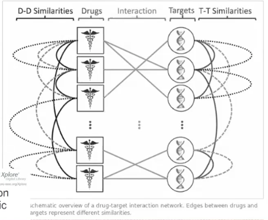
One particularly relevant example of such a complex relationship is predicting drug interactions. Say you have a collection of drugs. For some drugs, you may know what molecules they target, but for others, you do not. These relationships are indicated by the lines from drugs to targets. You may also have additional information about the relationship between the drugs' chemical forms, for example, that two drugs may be chemically similar. These relationships are indicated by the lines between drugs.
Given these known relationships between drugs and targets, you wish to be able to predict whether other two drugs may hit the same target. You also may be interested in whether a particular drug can be repurposed to hit a new target. We cannot answer this problem using simple multiclass classification - instead we wish to model all of specific relationships between each drug and each target.

Example: Information Retrieval

Another example is information retrieval. A particularly famous example of using graphical models to represent relationships would be Google's Pagerank algorithm; more generally, graphical models can model all relationships between elements in a knowledge graph.

Graphical Models

The purpose of a graphical model is to create a visual and structured representation of the probabilistic relationships in a given problem formulation. Graphical models help us visualize models, communicate about models, and consolidate all relevant information about a model. To construct graphical models, we introduce a notational system to unambiguously convey a problem setup.
We've already been informally drawing graphical models for a long time! For example,
The first graph on the far left represents a generative process where labels $y$ are used to generate features $x$.

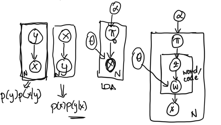
The second graph from the left represents a probabilistic process where labels $y$ are assigned a probability given features $x$.

The third and fourth graphs from the left are used to represent simplified and expanded versions of LDA.

Notation and Rules

Now, let's discuss the system of rules by which graphical models are created. These 4 simple rules will enable you to easily interpret graphical models and create your own graphical models!

1. Random variables are represented by an open circle. If we observe a random variable of a given model, then we shade it in. Otherwise, it's left open.
2. Deterministic parameters are represented by a tight, small dot.
3. Arrows indicate the probabilistic dependence relationship between different random variables and parameters. An arrow from $X$ to $Y$ means that $Y$ depends on $X$.
4. Plates, or boxes, indicate repeated sets of variables. Often there will be a number in one of the corners indicating how many times that variable is repeated. For example, if you have a training dataset of $N$ random variables $\{x_i, y_i\}_{i = 1}^{N}$ drawn from $X, Y$, you can draw a plate around $X$ and $Y$ in your model with an $N$ in the corner.

Dependency and Factoring

Rule 3 suggests that we can examine a sequence of arrows in a graphical model as a chain of dependencies of the random variables they connect. From examining the dependencies in graphical models, we can learn how to factor the joint probability distribution over all random variables in the graphical model.
Let's bring back the picture of the graphical models from above:
Let's first examine the first graphical model from the left. For this model, the joint probability distribution over all variables is: $$p(X, Y)$$ Which, using the dependency structure given in the graphical model, we can factor into $$= p(Y) p(X | Y)$$ In contrast, for the graphical model that is second from the left, we can factor the joint distribution into $$p(X, Y) = p(X) p(Y | X)$$ Similarly, for the simple LDA model (third from the left), we can write the joint distribution as $$p(\pi, x, \theta, \alpha) = p(\alpha) p(\theta) p(\pi | \alpha) p(x | \theta, \pi)$$ This factorization follows intuitively from looking at the graph: because there are arrows from $\theta$ and $\pi$ to $x$, then $x$'s distribution must be conditioned on (or dependent on) $\theta$ and $\pi$.

For the expanded LDA model (fourth from the left), we can write the joint distribution as $$p(\alpha, \theta, \pi, z, w, x) = p(\theta) p(\alpha) p(\pi | \alpha) p(z | \pi) p(w | z, \theta) p( x | w)$$
A key point is that while graphical models can tell us important information about the joint factorization of all of the random variables, graphical models do not give us the form of the distribution. Graphical models communicate dependencies between random variables, but do not indicate the distributions of the random variables themselves. For example, from observing the graphical model that is the first from the left, can we determine if $p(X, Y)$ is distributed normally? What is its mean and variance? Graphical models cannot capture this kind of information.

Bayesian Networks

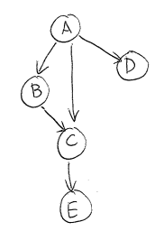
A Bayesian Network is a special kind of graphical model. Bayesian Networks (Bayes Nets) are DAGs (directed acyclic graphs) where nodes represent random variables, and directed arrows represent dependency relationships between random variables.
For example, the joint distribution of random variables $(A, B, C, D, E)$ can be inferred from the dependency relationships specified by this Bayes Net: $$p(A, B, C, D, E) = p(A) p(D | A) p(B | A) p(C | A, B) p(E | C)$$ Notice that even without any knowledge of the dependency relationships between the variables, we could always factor the joint distribution as $$p(A, B, C, D, E) = p(A) p(B | A) p(C | B, A) p(D | C, B, A) p( E | D, C, B, A)$$ But additional knowledge from our Bayes Net of the dependencies between variables allows us to write a simpler expression where several terms are conditioned on fewer variables. For example, our Bayes Net tells us that term $ p( E | D, C, B, A)$ can be simplified to $p(E | C)$.

Why are Bayes Nets, and the additional structure they provide to reason about dependency relationships between variables, useful?

1. For inference: if our goal is to fit some of the variables, given others, then we can do block coordinate ascent or alternating optimization schemes.
   
   For example in Figure 2, given $C$, $E$ becomes independent of all other random variables in the network.
   
   Therefore a possible inference scheme is to first guess that $C = c$. Given this guess of $C$, now we can update our guesses of $A, B, D$ and $E$. Then, given these guesses for $A$, $B$, $D$, and $E$, we now can update our guess of $C$. We can continue ``swapping'' between updating our guesses of these two groups of variables.
   
   
2. For learning: Bayes Nets allow us to learn ``smaller'' distributions, or distributions with fewer parameters.
   
   For example, before the joint distribution for the network in Figure 2 is simplified, $p(E | D, C, B, A)$ is dependent on $\{A, B, C, D\}$. If each of $\{A, B, C, D\}$ is binary, then there are 16 different ``settings'' of $p(E | D, C, B, A)$; for example $p(E | D = 0, C = 0, B= 0, A = 0)$, $P(E | D = 1, C = 0, B= 0, A = 0)$, etc. As such, we require 16 different ``parameters'', or terms $p(E | D, C, B, A)$, to fully specify the distribution.
   
   However, once simplified this term to $p(E | C)$, we only need to learn $p(E | C = 0)$ and $p(E | C = 1)$ to fully specify the distribution $p(E | C)$.
   
   

Intuition for D-separation

First we'll informally explore how conditioning on random variables may affect dependency, using this Bayes Net as an example: We will begin by defining the principle of local independence: every node is conditionally independent of its non-descendants, given only its parents.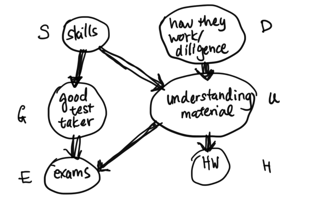

Example: Given $G$ and $U$, $E \perp H, S, D$ (or $E$ is conditionally independent ($\perp$) of $H$, $S$, and $D$).

Q: Given $S$, are $G$ and $U$ independent?
A: Yes: local independence says that $G$ and $U$, which are non-descendants, are independent given their parent $S$.

Q: Given $E$, are $G$ and $U$ independent?
A: No. First notice here that we cannot apply the principle of local independence, because $E$ is not a parent of $G$ or $U$.

Intuitively, if you know that someone did really well on their exam, and you find out that they really understood the material, then you may have less idea of whether or not they are a good test taker, because knowing that they really understood the material already ``explains'' their high performance on the exam. Therefore conditioned on observing the student's exam score, understanding the material and being a good test taker are dependent variables. This general phenomenon is called the explaining-away effect.

The D-separation Rules

When discussing D-separation, we use the term ``information flow'' to describe dependencies between variables. If there is information flowing from $A$ to $B$, then $A$ and $B$ are conditionally dependent given the observed random variables. In contrast, if $A$ and $B$ are ``blocked'', then $A$ and $B$ are conditionally independent given the observed random variables.

Two variables $A$ and $B$ are D-separated, or independent, if every undirected path from $A$ to $B$ is ``blocked''.

There are 3 base cases to determining if a path is ``blocked'':
Case 1:

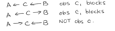
In Case 1, if we have observed $C$, then $A$, which is a descendant, will be independent of $B$ (by local independence).

Case 2:

In Case 2, $C$ is the parent of both $A$ and $B$. Because $A$ and $B$ are non-descendents, $A$ and $B$'s conditional independence follows by local independence.

Another contextualized example is: say $C$ represents the bias of a coin. $A$ and $B$ represent two independent flips of the coin. When $C$ is unobserved, then $A$ and $B$ are dependent, as observing the result of flip $A$ may give information about the bias $C$ of the coin, which also gives information about $B$. But once $C$, the bias of the coin, is observed, then $A$ is now independent of $B$.

Case 3:

In Case 3, not observing C blocks the path. When C is observed, it induces a correlation, or dependency between $A$ and $B$.
An example of this is $C$ being the XOR of $A$ and $B$. When $C$ is unobserved, $A$ and $B$ are uncorrelated. But once $C$ is observed, $B$ can be calculated from observing $A$ and $C$.

Section 8.2.5 of the textbook discusses each of these D-separation rules more in-depth, we strongly recommend that you read it as a supplement to this lecture!

Uniqueness and Parameters

Uniqueness

Mathematically, it is true that given any two random variables $(A, B)$, we can write the join distribution $p(A, B)$ two ways: $$p(A, B) = p(A) p(B | A)$$ $$p(A, B) = p(B) p(A | B)$$ Each equation also has an associated ``ordering'':
Q: When factoring our Bayes Nets (or, more broadly, when factoring joint distributions in this course), which way should we choose, given that both of the above equations are mathematically correct?

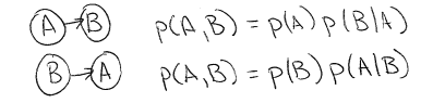
A: If we are given some causal knowledge, for example, if we know that $A$ causes $B$, then we should factor the joint distribution using $p(A, B) = p(A) p(B | A)$. We cannot ``flip the ordering'' under this causal assumption. Therefore in this case, there is 1 unique factorization that is consistent with our causal knowledge.

But otherwise, you can choose any factorization you'd like, given that the factorization is mathematically correct. However, some choices of the ordering are easier to work with than others.

Example: Ordering affects the number of necessary parameters

Example: Recall our network from Figure 3, here written using simplified variable names: Suppose all variables are binary. How many parameters does this network need? Or, otherwise stated, how many different values do we need to know to be able to calculate the joint distribution $p(S = s, D = d, G = g, U = u, E = e, H = h)$ for all possible values $s, d, g, u, e, h \in \{0, 1\}$?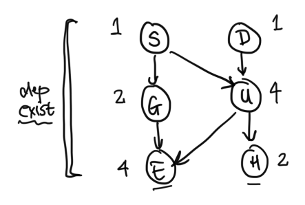

First, notice that $p(S)$ can be fully specified by $1$ parameter, as $p(S = 0) = 1- p(S = 1)$.

Similarly, $p(G | S)$ can be fully specified by $2$ parameters $p(G = 1 | S = 0)$ and $p(G = 1 | S = 1)$, as $p(G = 0 | S = 0) = 1 - p(G = 1 | S = 0)$, etc.

It is a good exercise to reason about the number of parameters required for each term in the joint distribution for our Bayes Net. In Figure 6, we've written the number of necessary parameters for each variable's conditional distribution term next to the variable. Therefore the network needs $$1 + 2 + 4 + 1 + 4 + 2 = 14$$ total parameters.

Creating a re-ordered network

We can change the topology (ordering) of the net, while preserving the same dependency relationships between variables. For example, this net has a re-ordered topology, preserving the relationships above: This network was created by thinking of the original Bayes Net in Figure 6 instead as a generative process. Say that we wish to place $E$ at the top of the network. Now, we consider $H$. Can $H$ be chosen independently of $E$ in the original network? No, because their parent $U$ has not been observed, and so there is an unblocked path $(E, U, H)$ between them. Therefore we need an arrow from $E$ to $H$.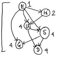

Now, we add $U$ to the new network. $U$ is not independent of $E$ or $H$, so we need to draw arrows from $E$ and $H$ to $U$.

Now, we add $S$ to the new network. $S$ depends on $U$ and $E$ because we have not observed $G$ yet. Because $U$ has been observed, blocking all paths from $S$ to $H$, we do not draw an arrow from $H$ to $S$.

Now, we add $G$ to the network. $G$ depends on $E$ and $S$, so we draw arrows from $E$ and $S$ to $G$.

This new network in Figure 7 respects all the dependencies of the original network in Figure 6. Note that the new network contains more dependencies (or arrows) than our original network.

Our new network in Figure 7 has 19 required parameters. It requires more parameters than our original network.

We could always write out a network in any arbitrary order, where every variable is connected to every previously added variable, and create a fully-connected graph representation: This network corresponds to factoring the joint distribution as $$p(E, S, U, H, G, D) = p(E) p(S | E) p(U | E, S) ...$$ While such an ordering is correct, it is not parsimonious. Our hope is to find a variable ordering which respects all necessary dependency relationships, while using as few ``arrows'' or having as few dependencies as possible. Generally, adding another arrow or dependency to a Bayes Net will increase the number of parameters required to specify the full joint distribution. As such, networks that have fewer arrows but still preserve the original dependency relationships will require fewer parameters to specify their joint distributions.

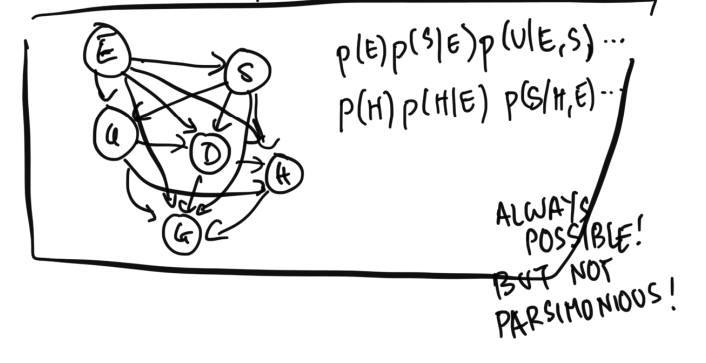
This fully-connected graph requires $1 + 2 + 4 + 8 + 16 + 32 = 63$ parameters.

Student question: What does the direction of the arrows imply? Do the arrows inform us of how the data is generated? In the top image, for example, $G$ and $U$ points to $E$. In the bottom image, $E$ points to $H$ and $U$.

Answer: You are correct in that it is possible to draw two Bayes Nets that preserve the dependency relationships between variables, but, because of their differing structure, tell a different ``story'' about each random variable in the network. This relates to the ``Uniqueness and Parameters'' discussion above. Typically, you wish to draw a graphical model that corresponds with your knowledge and your assumptions about a causal or data-generating process.

To contextualize our examples, in Figure 6, $G$ and $U$ point to $E$. The joint distribution of this Bayes Net can be factored as $$p(S) p(D) p(G | S) p(U | S, D) p(E | G, D) p (H | U)$$ This would represent a causal setting where we assume that being a good test taker and understanding material causes one's exam score.
In contrast, the Bayes Net in Figure 7 can be factored as $$p(E) p(H | E) p(U | E, H) p(D | U, S) p(G | S, E) p (S | U, H)$$ This factorization may be helpful in a setting where a student's exam score is observed, and a researcher is trying to learn student profiles (their $H$ and $U$) from exam scores.

Beyond Bayes Nets

In CS 181, we are only going to focus on Bayesian Networks. But, there are more kinds of graphical models out there! We'll briefly introduce two other kinds of graphical models.

Undirected Models

Undirected models are graphs where the edges between random variables are undirected. For example, consider graph The joint distribution of this graph can be factored as $$P(A, B, C, D, E) = \frac{1}{z} \phi(C, A, B) \phi(B, D) \phi(B, E)$$ where $z$ is a normalizing constant and $\phi$ is a function.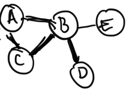

Undirected graphical models are very popular in settings such as image processing. In practice, they're hard to work with as normalizing constant $z$ is hard to find to make $P(A, B, C, D, E)$ a valid probability distribution which sums to $1$.

Factor Graphs

In factor graphs, variables connect into factors, which are denoted by the shaded nodes: The joint distribution of the factor graph can be written as $$p(A, B, C, D, E) = \frac{1}{z} \phi(B, D) \phi(B, E) \phi(A, B, C) \phi(B, C)$$ where $z$ is a normalizing constant and $\phi$ is a function.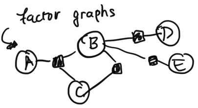

Each of the $\phi()$ terms was created by examining each of the factor nodes, and including the variables which were connected to each factor.

Factor graphs are more expressive than undirected graphs. Notice here that we included a factor to add additional term $\phi(B, C)$. Notice that we wouldn't have been able to specify the inclusion of this extra term in our undirected graphical model.