Date: February 10, 2020 (Concept Check, Class Responses, Solutions)

Relevant Textbook Sections: 3.6

Cube: Supervised, Discrete, Probabilistic

Lecture 5 Summary

• Re-intro to Classification: Real World Applications of Classification
• Intro to Probabilistic Classification
• Discriminative Approach
• Generative Approach

Relevant Videos

• Gradient descent
• Logistic Regression
• Generative Classification

Re-intro to Classification: Real World Applications

In the previous lecture on linear classification, we didn't get a chance to cover some real world motivations of classification yet. We start this lecture motivating a couple of quick examples. First, in the context of fraud, we want to be able to classify emails as spam or not spam. In the study of birds, there are some scenarios where based off audio, we want to be able to classify wwhat bird the audio represents.

Is is also important to keep real world considerations in mind when designing systems of prediction. In the past, classification was once done on tumors, to tell tumors are benign or malignant (for breast cancer). Initially, it worked, and the system was so good that the government paid hospitals to use the classification system. However, after everyone started using the system, research found that the doctor's with the classification tool did worse than those without the tool. It turned out that during the original study, the doctors actually had the time to look at the system carefully and used their expertise knowledge in conjunction with the prediction output to make better predictions. However, once it was incorporated into doctor's daily routines, they didn't have enough time to use both use personal expertise and considered the just system's output heavily, leading to worse performance. It is important to keep real world considerations in mind as we create and apply these prediction systems in life.

Intro to Probabilistic Classification

Last lecture, we covered linear classification, from a nonprobabilistic view. Specifically, we had a rule, $sign(w^Tx)$ when we used labels y=1 and y=-1, (or $w^Tx$ with a boundary of 0.5 if we used labels y=1 and y=0). There no notion of probability anywhere, and in our binary classifier that we looked at, we essentially said: if we were on one side of the boundary, it was definitely one class, and if we were on the other side of the boundary, it was definitely the other class.

Today, we cover probabilistic modeling, where we want probability that a particular input belongs to a particular class. For example, perhaps you had a photo of both a dog and cat, and the classififer isn't sure if it a dog or a cat. Ideally, we'd want a classifier that is able to tell if it's unclear, and assign some probability to each of the two possibilities. One of the reasons we'd want this is because using probabilities is great for decision making. If you know the penalty of a false positive versus a false negative, for example, you can now compute an expected value, and you can use this information to do calibration on your model.

Within probabilistic classification, there are two different approaches to the problem: discriminative and generative.

Discriminative Approach (Logistic Regression)

First, we'll look at the discriminative approach. This means that we are tackling $p(y = C_k | x_n)$ directly. Essentially, we want a function for $p(y = C_k | x_n)$ of $x_n$ that turns it into a probability (since now we are doing probabilistic classification). To do this, we choose sigmoid function as a tool to use in our model: $\sigma(z) = 1/(1 + \exp(z))$ (will discuss later).

Remember first, the big picture steps of setting up a model.

1. Choose a model class, as in a type of boundary (today: linear)
2. Choose a loss function (today: logistic loss)
3. Optimize for w*

Note: logistic regression, while called logistic, is considered a linear model because we linearlly multiply the weights with the x.

1. Choose our model class (we chose $\sigma(-w^Tx)$ specifically)

Since we have a linear model, we start with some notion of $z = w^Tx$. Next, we use our sigmoid function that we discussed earlier. The reason we choose to a sigmoid function is mainly convenience. There is no special meaning to why values should be mapped to probabilities specifically in the form of sigmoid, but it is very nice because it returns values between 0 and 1, and essentially squashes our $w^Tx$ into an easy to work with probability.

So our final function is as follows: $$\hat{p}(y=1 | x) = 1/(1 + \exp(-w^Tx))$$ Since we are in a binary case, we can also easily calculate the probability of y=0 given x. $$\hat{p}(y=0 | x) = 1 - \hat{p}(y = 1 | x) = 1/(1 + \exp(w^Tx))$$ To give more intuition on what sigmoid is doing, we see the following. At the boundary, $w^Tx = 0$, you end up with $1/(1 + \exp(0)) = 1/(1 + 1) = 0.5$, which makes sense because that is where we would assign 0.5 probability to each class. As the value of $w^Tx$ gets bigger, we think it's definitely more y=true. We again emphasize that this is the model we selected, we chose to use sigmoid for convenience and these are simply the properties that come up the sigmoid. It does seem to be intuitive for our simple case (but we coudl always select a different function that perhaps predicts y=1 with less certaintiy as $w^Tx$ increases to be too far away from the concentration of data).

This sigmoid concept can also be extended to the multiclass scenario by using the softmax function instead of the sigmoid function (intuitively, very similar idea, but for multiple classes). The softmax function essentially turns a vector of values into a vector of probabilities. This will be used in your homework.

Student Question: How often is sigmoid used? Always used pretty much. However, we can change what we input into the sigmoimd. It's just often easy to use since we need a squashing function at the endanyways to lead to probabilities of 0 and 1, and sigmoid is very convenient for this.

2. Loss function (logistic loss):

We pick a logistic loss, also known as a binary cross entropy loss. $$L(w) = -\sum_{n}y_n \log\hat{p}(y_n = 1 | x_n) + (1 - y_n)\log\hat{p}(y_n = 0 | x_n)$$ What is the intuition behind this loss? Essentially, we're trying to think about how much probability are we putting on the right answer. The more, the better, and the lower the loss. Note that here, $\hat{p}$ is our choice of our function from the above section, our prediction. Let's suppose the true label $y_n=1$, then we want the first term to be small since we want low loss. If we predict $\hat{p}=1$, then we're in great shape, beacuse 1*log(1) is 0. Then in the second term, we have (1 - 1) * log(0), which we evaluate to zero (while this is techincally undefined, in our logistic function's meaning, we want this to be 0 because we have predicted the right class). When coding for the homework, be careful as you may run into this issue! You would want to handle this case somehow (many ways to do it).

Student Question: How is logistic loss different from hinge loss? Hinge loss has y=0 from negative x until x=0, then it increases linearly. This means that hinge loss will stop as soon as everything is classified already, since as long as it's correct, it's satisfied and there is no loss. On the other hand, log loss will encourage us to move the line to be even better even though all the points are already classified correctly. This is because the distance to the boundary affects the probability we predict for a given point, so log loss considers it and continues to optimize.

3. Optimize for w*

We omitted this in lecture to save time. Essentially, what you would do here is gradient descent, by taking the derivative of the above loss (L(w)) with respect to w, and doing the following process:

$$\textbf{w}^{(t+1)} = \textbf{w}^{(t)} - \eta\frac{\partial \mathcal{L}(\textbf{w})}{\partial \textbf{w}}$$ We repeat until convergence, and we have our final optimal w*.

Generative Approach

Now we consider the generative approach. This means we now are interested in joint P(x, y) rather than p(y | x) which was the discrimanitive case above, logistic regression. What does this mean? Essentially, now we telling a generative story, specifically that y generates x. This is more complex in a way, but one big advantage is it can deal with missing data, or missing labels in a more elegant way.

In notation, this mean's we are now looking at these two terms. We sample y with some prior: p(y). Then, we sample x with some P(x|y).

So we know that we have a discrete output in y. Let's let y be binary and let p(y) be distributed Bernoulli with $\theta$, as in $p(y) = \theta^y(1-\theta)^{1-y}$.

Now we use Bayes' rule to rewrite: $P(y=C_k | x) \propto p(x | c_k) p(c_k)$

Where $P(y=C_k | x)$ is what we ultimmately want to maximize, but because of Bayes' rule its proportional to $p(x | c_k) p(c_k)$, so we can maximize that instead, where $p(x | c_k)$ is the proability that depends on the class, and $p(c_k)$ is the Bernoulli that discussed before.

Note: Having the $p(c_k)$ term there is important. This lets us model the base rate in the population. we can model that in the prior. Think to the syphillis example discussed in class. Even if a test returns positive for syphillis, we need to consider that the base rate of syphillis overall is so low that it's more likely that the test was wrong than a patient actually has syphillis.

Example of Generative Approach: Binary y and Gaussian x for Both Classes

1. Setting Up the Story

Let's say y is binary: $$y \sim \textrm{Bern}(\theta)$$ Let's say x is continuous. One way we can pick x is to pick a Gaussian distribution for both classes: $$x \propto N(\mu_1, \Sigma_1) \textrm{ if } y = 1$$ $$x \propto N(\mu_0, \Sigma_0) \textrm{ if } y = 0$$ 2. Minimizing Loss

We want to maximize p(y|x). $$p(y|x) \propto p(x, y)$$ $$p(y|x) \propto p(x|y)p(y)$$ $$\log(p(y|x)) \propto \log(p(x|y)) + \log(p(y))$$ So we can write our loss function as: $$L(w) = -\log(p(x|y)) + -\log(p(y))$$ 3. Calculating Optimal w*

For this particular example, we omit calculating the gradient of the loss and finding the optimal w*. To find it, you would do your usual gradient and the run gradient descent, plugging the p(x|y) and p(y) probabilities based off the story we set up (two Gaussians and Bernoulli respectively).

Let's analyze the boundary of this model to better understand it

Let us consider $\log(p(y = 1 | x)/p(y = 0 | x)) > 0$, the boundary.

Student Question: Why is this the boundary? This is the boundary because for log(z) to be greater than 0, z must be greater than 1. And here, z being greater than one simply means that the ratio of the probability of y=1 to the probability than y=0 is greater than 1. As you can see, if they are equal, as in both 0.5, then this term is exactly 0. And if the probability of y=0 is higher, than this term evalutes to less than 0.

To closely examine the boundary, we can plug in the actualy probability terms, and we reach the following: $$\log(\textrm{terms that don't depend on x}) - 1/2(x(\Sigma_1^{-1} - \Sigma_2^{-1})x^T - 2x(\Sigma_1^{-1}\mu_1^T - \Sigma_2^{-1}\mu_2^T) + \textrm{more no x terms}))$$ Why are we examining the boundary? Really, what we're trying to do here is build intuition on the impact of how we selected our distributions for x if y=0 and y=1. Here, we picked two Gaussians each with their own mean and covariances, and turns out the boundary looks something like above. If you look at the terms, you'll find that this boundary is going to be quadratic generally.

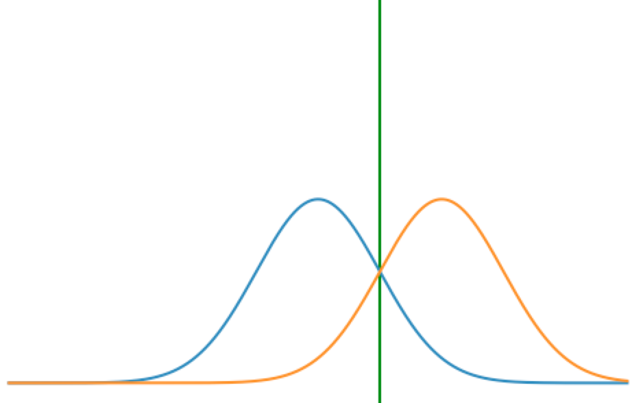
One super interesting exception though, is that if $\Sigma_1 = \Sigma_2$, then we have a linear boundary! First, let us show this mathematically from the equation.

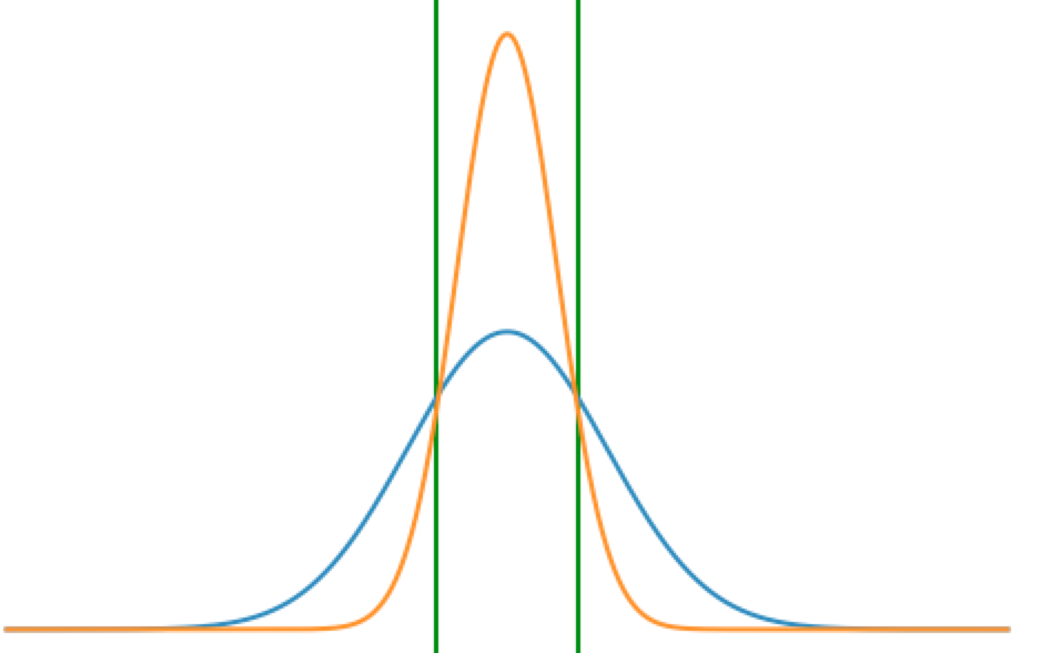
If we look above ignoring the terms that don't depend on x, and substitute in a $\Sigma_{same}$, we get: $$-1/2(x(\Sigma_{same}^{-1} - \Sigma_{same}^{-1})x^T - 2x(\Sigma_{same}^{-1}\mu_1^T - \Sigma_{same}^{-1}\mu_2^T)$$ $$-1/2(2x(\Sigma_{same}^{-1}\mu_1^T - \Sigma_{same}^{-1}\mu_2^T)$$ $$x \Sigma_{same}^{-1}(\mu_1 - \mu_2)^T$$ This, as you can see above, is a linear boundary. We can also give a visual interpretation, with a situation where x is only in one dimesion. Below first (left) is a graph of two Gaussians with the same variance. As you can see there is only one boundary (green) between which class is more likely (when you cross the line, you go from blue being the best guess to orange). Next (right) is a graph of two Gaussians with different varaince. As you can see, now there is one patch or region (denoted by green lines) where orange is a more likely class than blue, but on both ends of the patch, blue is more likely. This represents the quadratic situation.

What if x is discrete, not continuous?

All the above was done given the fact that x is continous. What's really beautiful about the generative set up here is that it's very easy to substitue in a new way of generating x's, as in subbing in a new p(x |y). Let's consider x now as discrete, and suppose we have d dimensions in, with each $x_d$ as binary.

Apply Naive Bayes Assumption To Make Life Easier: If the different dimensions are correlated, then we have up to 2^D paramaeters, as perhaps all the different cases ( as an example: 000, 001, 010, etc, if D=3) might have unique probabilities. One simplifying assumption that we can make (which might not be true) is the Naive Bayes assumption. Specifically, this assumes that y separately produces every element of the x vector (this is now part of our generative story). Essentially, given a class y, each x dimension is independently generated. Now, this means we just need D parameters.

Let us continue. Essentially, we can now reuse everything from above, except substitute in a new expression for $p(x|y)$. First, we know we've asssumed that the y generates the x in our story, so each datapoint is independent, and we start with: $$p(x|y) = \prod_n p(x_n|y)$$ We also now have the following, an even stronger assumption, due to the Naive Bayes assumption that each y generates each dimension of x independently as well: $$p(x_n|y) = \prod_d(p(x_{nd}|y))$$ We also know that the following holds: $$(p(x_{nd}|y)) = (\theta_{d,y=1}^{x_{nd}} (1 - \theta_{d,y=1}^{1 - x_{nd}}))^{\mathbb{1}(y_n = 1)} (\theta_{d,y=0}^{x_{nd}} (1 - \theta_{d,y=0}^{1 - x_{nd}}))^{\mathbb{1}(y_n = 0)}$$ To break down the equation above, first we recognize that at a high level, we have first the PMF of a Bernoulli ($\theta^x * (1-\theta)^{1-x}$) raised to the indicator variable of $y_n=1$, and then we have a PMF of a Bernoulli again raised to the indicator variable of $y_n=0$. This represents our story because this corresponds to the fact that we decided for both classes (y=1 and y=0), we have a binary variable for each dimension of x (binary corresponds to the Bernoulli).

Now, we can plug this into the final equation. $$p(x|y) = \prod_n p(x_n|y) = \prod_n \prod_d ((\theta_{d,y=1})^{x_{nd}} (1 - \theta_{d,y=1})^{1 - x_{nd}})^{\mathbb{1}(y_n = 1)} ((\theta_{d,y=0})^{x_{nd}} (1 - \theta_{d,y=0})^{1 - x_{nd}})^{\mathbb{1}(y_n = 0)}$$ Important note on indicator variables: this is a concept that shows up again and again, so definitely ask us if you don't completely understand. The reason we have this indicator variable raised to the exponent is because in the product across each of the n datapoints, we want to make sure we calculate the correct probability the current one of the n datapoints based of it's class. As in, for each n in the product, we only really want the first term, $((\theta_{d,y=1})^{x_{nd}} (1 - \theta_{d,y=1})^{1 - x_{nd}})^{\mathbb{1}(y_n = 1)} $, or the second term, $((\theta_{d,y=0})^{x_{nd}} (1 - \theta_{d,y=0})^{1 - x_{nd}})^{\mathbb{1}(y_n = 0)}$, we definitely don't want both since that doesn't make intuitive sense for one single datapoint. To make sure we only get one, we use indicator variables in the exponent, because if the indicator is 1, we keep the term (since some x to the power of 1 is still x), and if it's zero, we safely ignore the term (since some x to the power of 0 is 1, and when you multiply the existing product by 1 it stays the same).

Finally, what we notice is when we take the log of this equation, it leads to a clean looking result that can be used easily. And once you take the log, the product turns into a sum, and the indicator comes down from the exponent into a multiplicative term, which still works as expected! This is because, if the indicator is 1, we keep the term in the sum, and if the indicator is 0, we want to multiply out the term so that nothing (as in 0) is added to the sum, and the existing sum doesn't change.