Date: February 24, 2020 (Concept Check, Class Responses, Solutions)

Relevant Textbook Sections: 4.4, 4.6

Cube: Supervised, Discrete or Continuous, Nonprobabilistic

Lecture 8 Summary

• Intro and Motivation to Neural Networks
• Example: A Feed Forward Neural Network with One Hidden Layer
• Intuition 1: Universal Function Approximator
• Intuition 2: M of N Rules (and the power of neural networks)
• Architecture Choices

Intro and Motivation to Neural Networks

To start off the lecture, let us first do a intro into the topic of neural networks. Long story short, neural networks can be thought of as an extension of doing linear regression using a basis. In the past, we learned linear regression in the following form: $$\hat{y} = w^Tx$$ Because a linear model was often not enough to capture any complicated trends in the data, we made our model become more flexible by selecting a basis $\phi$. As an example, we might have had $\phi(x) = [1, x, x^2 ... x^j]$, $$\hat{y} = w^T\phi(x)$$ Our neural network extends on this basis regression process by adding a critical new idea: let's learn the basis. Because of this, neural networks actually used to be known as adaptive basis regression. At a high level, we want to learn this $\phi(x)$, so that instead of having to get an expert in some domain to figure out what a good basis should be for every different context, we instead learn it automatically.

It turns out, in practice, neural networks indeed work really well in the real world. One example is that in postal code sorting, neural networks are used to identify handwritten digits and thus mail can be automatically organized into the right buckets so that they go to the right places. Neural networks were also used to greatly improve the accuracy of Google Translate (while decreasing the size of the code base!). This doesn't mean Google Translate is perfect at translation (we all know that sometimes the translations don't work super well), but the fact was that the neural networks worked much better than the original method with less lines of code was a big deal. It is important to note however, that these neural networks will only be especially successful when there's lots of data available. Because of the European Union, there exists a lot of parallel datasets across different European languages, so those translations are done very well. In other areas, where there's smaller amounts of translation and annotation, the translations can be tough. Another common real world example of a neural network at work is face recognition software. Detecting a face is super common now (in our phone cameras, at immigration when you enter the country, etc). Again, as always, we want to be very careful when implementing these algorithms, as there are questions of quality that we should ask. As an example, are we making sure that all different colors of faces are identified at the same accuracy rate? Should we even have facial recognition software in certain contexts? How far should we go?

With that, let us move into the details.

Example: A Feed Forward Neural Network with One Hidden Layer

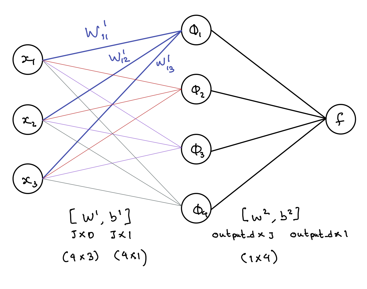
To start learning about neural networks, let us first start with an example, a feed forward neural network with one hidden layer. We have the following: a D dimensional input (D nodes in the input layer), a $\phi$ that transforms the input with D dimensions into an output with J dimensions (the one hidden layer with J nodes), and a 1 dimensional output (one output node f). In our diagram, we've chosen D to be 3, and J to be 4.

Let us all breakdown what's in the diagram below. First, in the leftmost layer of nodes, we have a bunch of D input dimensions. Next, between the input layer and the first hidden layer (the layer of $\phi$'s), we write out two parameters: $W^1$ and $b^1$. These parameters are drawn between the two layers because they serve exactly that purpose: to get us from our x input to the the hidden layer. How do we determine the dimensions of $W^1$? By convention, they will be J by D because the convention is to have the row as the dimension of the resulting layer and the column as the dimension of the starting layer (as you can see in the diagram, the dimensions work out in the math this way). In addition, we also have a J by 1 bias term $b^1$, where a given term represent a bias used for the creation of single one of the J nodes in the resulting hidden layer (see the equations in the diagram for the math). Next, let's look between the hidden layer and the output layer. Here, again, since we are between layers, we have parameters $W^2$ and $b^2$ here. The dimesions are 1 by J for $W^2$ since we are going from J dimensions to 1 dimension, and the $b^2$ has dimensions 1 by 1 since the resulting layer dimension is 1 (bias is always the dimesion of the resulting layer, by 1, since you only need one number for each of the nodes of the resulting next layer, and here, since our resulting layer is f that only has one dimension, $b^2$ is literally just a number).

Note: this architecture is called a feed foward neural network because there are no cycles formed betwen the nodes. The equations below correspond with the graph above, where x here represents a single datapoint with d dimensions. $$f = W^2\phi(x) + b^2$$ $$\phi(x) = \sigma(W^1x + b^1)$$ We also write this in matrix form. Essentially this is how to apply $\phi$ to an input x. The sigmoid is applied row wise after doing the computation inside. $$\phi(x) = \sigma\left(\begin{pmatrix} W^1_{11} & W^1_{12} & W^1_{13} \\ W^1_{21} & W^1_{22} & W^1_{23} \\ W^1_{31} & W^1_{32} & W^1_{33} \\ W^1_{41} & W^1_{42} & W^1_{43} \\ \end{pmatrix} \begin{pmatrix} x_{1} \\ x_{2} \\ x_{3} \\ \end{pmatrix} + \begin{pmatrix} b^1_{1} \\ b^1_{2} \\ b^1_{3} \\ b^1_{4} \\ \end{pmatrix} \right) $$ With matrix form, we can now do the literal math out and see an example of how the first element of $\phi$ is generated, as an example. This is depicted in dark blue, and the math is as follows: $$\phi_1 = \sigma(W^1_{11}x_1 + W^1_{12}x_2 + W^1_{13}x_3 + b^1_1)$$ Note that we don't depict the bias in the diagram. There is basically also one bias term applied to each of the J $\phi$ terms.

Student Question: Why do we name the output node f, and not $\hat{y}$? We name this f and not $\hat{y}$ because we are keeping our expression general enough to be used for either of both classification and regression. This means, if we use it for classification, we could feed it into a sigmoid function (note: we are only working with a one node output layer, so we can only do binary classification which is achieved with sigmoid), and end up with $\hat{y} = \sigma(f) = \sigma(w^T\phi + w_0)$, and then we could use the result to convert the number into a class (if we were doing multiclass, we would need multiple output nodes in the output layer, and then apply softmax, for example). If used for regression (note: it has to be a one dimensional y here because again, we only have one output), then yes, f wouldn't need to be passed through $\sigma$, $\hat{y}$ would directly equal f.

Student Question: Why do we select $\sigma$ to be in the function $\phi$? This choice of function that we apply on to the $wx + b$ term is called the activation function. It's very important that we picked $\sigma$, a nonlinear function (there are other nonlinear functions but $\sigma$ is a common one), as the nonlinearity is what makes our neural network model more sophisticated than a simple linear regression. To really visualize this, we can try setting $\phi$ to simply be the linear combination $wx + b$, and we can see what happens when we don't add in a nonlinear activation function. We start with $\phi(x) = W^1x + b^1$ (no sigmoid function this time) and $f = W^2\phi(x) + b^2$. This means now that we have $f = W^2(W^1x + b^1) + b^2$ which simplifies to $f = W^2W^1x + (W^2b^1 + b^1)$. As you might've noticed by now, it turns out that our result when we don't use a nonlinear activation function, is we end up with just another lienar regression in the end, with W set to $W^2W^1$ and b set to $W^2b^1 + b^1$. So this is why we select a nonlinear activation function!

Intuition 1: Universal Function Approximator

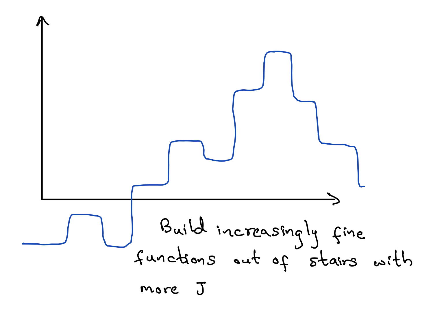
So with this set up, what are we able to model anyways? Does it even work? Turns out, we can model a lot! For a big enough J (as in, if that hidden layer has enough nodes), this is actually a universal function approximator! To get some intuition behind this, imagine first the J=2 scenario picking sigmoid as our activation function. Essentially, what we can do is build up a little staircase like figure below, with the sigmoid functions together.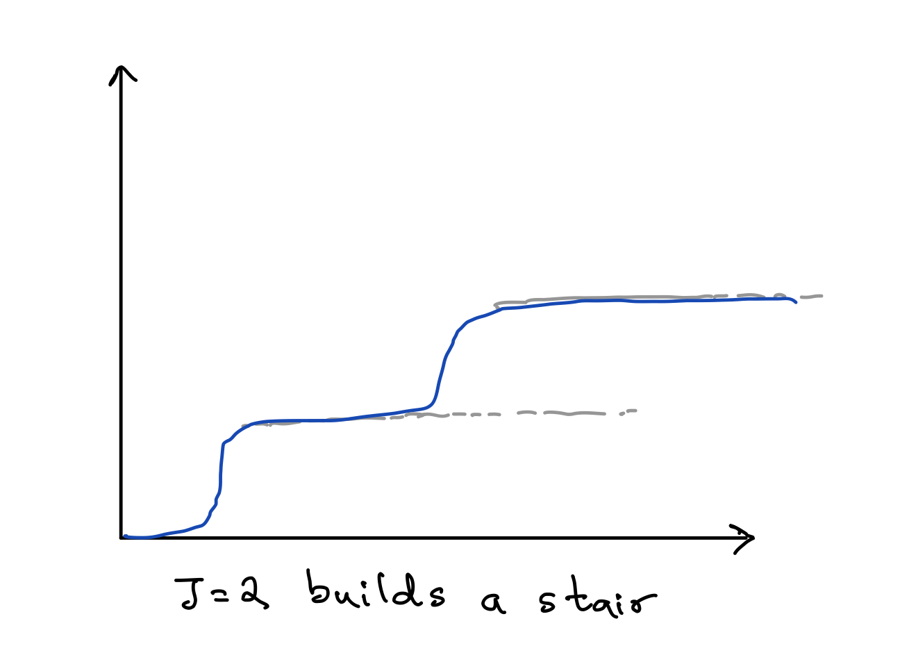 As we have more and more sigmoid functions (which we get when we add more nodes to the hidden layer), we can represent increasingly complicated functions, as if we have a really fine staircase. Note: this also helps us realize the limitations of this approach! Now, even representing a simple line $f = w^Tx + b$ will be hard, as we will need lots of little steps in the staircase to produce a smooth looking line.

Activation Functions: What can we use instead of sigmoid?

We can also use these other nonlinear activation functions: the ReLu function, the leaky ReLu function, the tanh function, and the radial basis function. And for all these functions, it turns out that still, for a big enough J, they're also universal function approximators!

Intuition 2: M of N Rules (and the power of neural networks)

Imagine we have a scenario where we want to map the not XOR function. This means, if we have inputs x=[0, 1] or x=[1, 0], we want an output of y=0, and if we have inputs x=[1, 1], or x=[0, 0], we want y=1. Turns out, there's no way to draw a single line to separate the data with full accuracy. Now we can leverage the power of neural networks (and we can think if the power through the M of N rules, which will be explained at the bottom).

Let's look at the exact four x datapoints we mentioned above, x=[0, 1], x=[1, 0], x=[1, 1], and x=[0, 0], and see what we can do.

Here is an example neural network setup that would be able to distinguish these points. Note: this is a little different from lecture as in lecture there is a lot of content to cover in a small amount of time. Here, we've edited it because we actually did all the literal number substituions and found that these numbers are a bit more easy to reaosn with.

Let's say we have $f = \phi_1 + \phi_2$ where if f is greater than or equal to 0.77, we classify the point as y=1, and if f is less than 0.77, we classify the point as y=0. We define $\phi_1$ and $\phi_2$ below $$\phi_1 = \sigma(-x_1 - x_2 + 0.5)$$ $$\phi_2 = \sigma(x_1 + x_2 - 1.5)$$ In a story sense, we're basically saying, if either of $\phi_1$ or $\phi_2$ are "on" (as in largely positive), then the final result of f will be bigger, and if it's bigger than 0.77 (a threshold we set that divides the points), we'll classify it as y=1. For the graphical interpretation on this, we can look at the term inside of each $\phi$'s $\sigma$. For $\phi_1$, we can look at $-x_1 - x_2 + 0.5 > 0$ (since if it's greater than 0, $\sigma$ of something positive will return something larger than 0.5 which is on the larger side, which we can say is "on"). If we rearrange this, we get $-x_2 < -x_1 0.5$. Basically, the more below we are to this line, the more positive the overall $\phi_1$ gets. So we see how $\phi_1$ is picking out the point [0, 0] and turning $\phi_1$ "on" (making it pretty positive) when we see [0, 0]. $\phi_2$ does the exact same thing on the other side. Let's rearrange the term inside. $x_1 + x_2 - 1.5 > 0$ can be rewritten as $x_2 > 1.5 - x_1$ showing how anything above that line depicted in the graph will lead to a higher value of $\phi_2$, turning it "on".

Let's literally through all four points' math for more intuition, before we fully tie this into the M of N rules intuition.

x = [0, 1]

$$\phi_1 = \sigma(-0 - 1 + 0.5) = 0.377$$ $$\phi_2 = \sigma(0 + 1 - 1.5) = 0.377$$

x = [1, 0]

$$\phi_1 = \sigma(-1 - 0 + 0.5) = 0.377$$ $$\phi_2 = \sigma(1 + 0 - 1.5) = 0.377$$

x = [0, 0]

$$\phi_1 = \sigma(-0 - 0 + 0.5) = 0.622$$ $$\phi_2 = \sigma(0 + 0 - 1.5) = 0.18$$

x = [1, 1]

$$\phi_1 = \sigma(-1 - 1 + 0.5) = 0.18$$ $$\phi_2 = \sigma(1 + 1 - 1.5) = 0.622$$

Full Intuition of M of N Rules

Overall this shows how we have M of N rules (and this occurs at multiple levels). First, at the level of $\phi$, we have the following: for $\phi_1$, it's "activated" when M of N rules are met, specifically with M=2 of N=2 in our case. For $\phi_1$ we see that if both $x_1$ and $x_2$ are 0 (our two rules), we then get an "activated", pretty positive $\phi_1$ result which we calculated to be $\sigma(0.5) = 0.622$ (pretty high). If either of $x_1$ or $x_2$ didn't follow the rule and one of them or both of them weren't 0, we would see that the result would no longer be "on" and would be "off" instead (see numbers we calculated above: we got 0.377, 0.377 and 0.18 for [0,1], [1,0] and [1, 1]). Note: these two rules of having both $x_1$ and $x_2$ as 0 can also be described as the graphical interpretation given above (namely, requiring that $x_1$ and $x_2$ leads to a point below the line that $\phi_1$ plots).

The same applies to $\phi_2$. It also asks for 2 of 2 rules to be met, but the rules for this one are that $x_1$ is 1 and $x_2$ is 1. If either of them is 0, the final result of $\phi_2$ would become $\sigma$ of a negative number, and that would turn it "off".

Next, we jump to the next level. At the f level, we also have M of N rules. Specifically, we want 1 of 2 rules to be met to get our y=1 final label. Our rule is whether a given $\phi$ is "on". By having at least one "on" (essentially having at least one big number), based off the way we set up the equations an the threshold, this pushes us over the threshold, leading to the final classification of y=1. If we don't meet our at least 1 of 2 rule, and we have both numbers as "off" (in this case, that would mean $\phi_1=0.377$ and $\phi_2=0.377$ as we calculated above), then we're not big enough to meet the threshold and hence classify the input as y=0.

Architecture Choices

As you may have noticed, the structures of the neural network in our first example and the neural network in the classification example were different. The first simply had one $\phi$ function that transitioned us from the input to the hidden layer using a sigmoid function, a J by D $W^1$ matrix, and a bunch of other parameters. Whereas the other had two $\phi$ functions that took the sigmoid of x inputs that were just summed or subtracted (and along with a constant), and then the $\phi$ functions were summed at the end to produce the final f. There are a lot of neural network strutures. Here are some others:

Deep Neural Network

This is an extension of what was drawn before. Basically, a deep neural network is a feed forward neural network with multiple hidden layers. Between layers, there are still the [W and b] terms, as we drew on our diagram before as well.

Why would we do this if a single layer is a universal function approximater? We would want to do this if we need to reuse parts of structure. Imagine a situation where we wanted it to be:

$$ \textrm{output=true if either} \left\{ \begin{array}{cc} \textrm{x1 and x2 and x3 are big} \\ \textrm{x1 and x2 and x4 are big} \\ \end{array} \right. $$ If we set it up with just one hidden layer, we would be relearning the x1 and x2 parts, which really we could combine into a resuable term (x1 AND x2). So instead, let's set it up in the following way for computional efficiency: $$ \textrm{output=true if either} \left\{ \begin{array}{cc} \textrm{(x1 and x2 are big) AND x3 is big} \\ \textrm{(x1 and x2 are big) AND x4 is big} \\ \end{array} \right. $$ This way, in one of our $\phi$'s we can first figure out (x1 AND x2) and then reuse this.

Other Architectures

There are a lot of other architectures of neural networks. Finale covered the basic intuition in class for each of these, but we encourage you to do your own research (explore websites, videos) to find out more, rather than just write a simple sentence for each. If you have any questions, of course feel free to reach out to us on Piazza or email jdhe@college.harvard.edu, and if there's enough demand, we can add in more notes here.

• Residual Network (Variant of a Feed Forward Network)
• Convolutional Network
• Auto-encoder
• Recurrent