Date: April 22, 2020 (Lecture Video, iPad Notes)
Lecture 22 Summary
- Intro: Reinforcement Learning in the World
- Back to Value-Based Approaches
- Deep Q-Network (Approach 1 for Value-Based Continuous)
- Fitted-Q Iteration (Approach 2 for Value-Based Continuous)
- All Three Methods (Value-based, Policy-based, Model-based)
- Optional Material
Intro: Reinforcement Learning in the World
In reinforcement learning, we've seen how it's hard to transfer things into the real world, especially with regards to how we define our reward functions. However, one application of RL that has developed a lot is in the context of playing games. This is because the rules and objectives are clear.In the past, we thought that if we could make an AI play games really well, then it means we've created something that is smarter than humans and that was quite exciting at the time. Nowawadays, we've categorized AI's that can play games well as part of "Narrow AI", which is defined as AI that's programmed to do a single task (such as play a game, check the weather, etc), to be distinguished from "General AI", which refers to machines that exhibit actual human intelligence.
Despite this, it is still important to think through the evolution of Narrow AI, as this will highlight some of the technical challenges that were overcome for us to be able to play games well.
One application of RL in games was in Backgammaon (Gerald Tesauro). This was the first time an AI got to a world class expert level of performance, and the AI was an artificial neural net trained by a form of temporal difference (TD) learning, something we covered in last class. Because it used TD, the AI was named TD-Gammon. A more recent breakthrough took place in 2013, where DeepMind was able to master several atari games (a set of games including video pinball, breakout, robotank, crazy climber, and more). Next, we had AlphaGo. Something that's interesting about AlphaGo is just how differently Go was solved compared to a gamel like chess (DeepBlue). Whereas DeepBlue used a traditional method of doing a very deep search into the future (by considering if I do this, they'll do that, then if I do this, etc), in Go, it's simply impossible to search far enough. We can't even come close to bottoming out the game, and so instead, AlphaGo did some searching to some depth but then from that point onwards, learned if this "type" of game position was good to do this sort of move, or this other sort of move. It essentially developed a heuristic of good board positions vs bad positions, and over many many games played with itself, it eventually defeated the human Go world champion.
Back to Value-Based Approaches
As a quick recap from last lecture, we mentioned there are three groups of approaches of doing reinforcement learning. We didn't finish our first group yet, our value-based methods, so we continue that today.Specifically, last class we were looking at value-based methods for discrete state and action spaces. This lecture began with a long recap of last lecture, to make sure students were on the same page with regards to understanding. See time stamp 15:23 to 42:53 for the review. In the review, Finale also added one additional off-policy example to our value-based approaches in discrete space, which we cover below:
Concluding Discrete Spaces with One More Off Policy Example
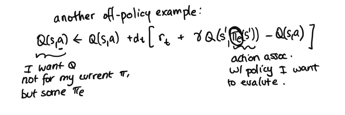
Last class, we covered an on policy example (SARSA), and an off policy example (Q Learning) as part of our value-based approaches in discrete spaces. We intorduce one more example of an off policy example.Imagine you're in a scenario where you know that there is a good policy out there. In the medical context, for example, there might be some well-researched policy that is good to follow for how to treat a patient. The key difference then, is our a', the same difference we saw between SARSA vs Q-learning. Where in SARSA, we used the a' from looking at our history and grabbing what action we actually took following our policy, and whereas in Q-learning, we used the argmax, as in the best $a^*$ of all the possible actions to exit $s'$, now we take a predefined policy when taking considering the which $a'$. As in, we have our external policy $\pi$, and we get our a' by doing $a' = \pi(s')$. Screenshot of math is below:
Continuous Space
So far, our value based methods for RL have been in discrete settings. Some might ask: why bother covering discrete settings like GridWorld? Doing GridWorld seemspointless and unapplicable in the real world. However, the reason it's important to cover gridworld is becaue while unapplicable, it builds very solid intuition for RL algorithms in general. The things that go wrong in simple settings still can go wrong in complex settings, so it's important for us to nail the simpler settings first.The biggest difference between discrete and continuous settings is that now, our Q Table can't exist because it's continuous: we cant just hold a table of states by actions. How can we replicate the Q(s,a) from SARSA and Q-Learning? We need to approxmiate Q(s, a) with some function class: for example, a deep network. We also still need to be able to learn the Q(s, a) function given histories. Below are two approaches:
Deep Q-Network (Approach 1 for Continuous)
We can use a neural network to approximate the Q-value function. This started getting popularized in 2013 and onwards. Let's say for example that we want to implement SARSA in our Deep Q-Network, which means we're given tuples of $(s, a, r, s', a')$ that are pulled from the history. Then, we can set up the following loss equation (W represents the weights of the neural network). (Note: Deep Q-Network can be done with the Q-Learning approach, just change the $Q(s'_n, a'_n)$ below accordingly to $max_{a^*} Q(s'_n, a^*)$, the same difference as in our discrete settings). $$\sum_n (Q(s_n, a_n) - [r(s_n, a_n) + \gamma Q_W(s'_n, a'_n)])^2$$ In this equation, the inside, $Q(s_n, a_n) - [r(s_n, a_n) + \gamma Q_W(s'_n, a'_n)]$ represents the temporal difference error.Our Goal: Learn the $Q_W(s, a)$ that minimizes TD error on the data we have (and we'll still use $\epsilon$-greedy for picking our actions).
The idea here is that we first collect some data, taking actions by following our policy. Over time, we'll have our experience tuples from our history, and given those tuples, we want to train a Q function that minimizes this loss. Specifically, we are optimizing the loss with respect to the W weights in the neural network that we use to approximate the Q function.
Note: we could update after each action, but usually we update from the history after some actions.
In practice, a few things are very tricky:
1. Choose what mini-batches of history to update with
The reason this becomes a challenge is that by doing function approximation, we now have the opportunity to forget. When we were in our discrete state action space, the $Q(s, a)$ was literally a number sitting there in a matrix, it didn't matter if you didn't touch it, you would always remember if a given state action pair is really bad, for example. But when we do an approximation, especially when taking a mini-batched approach, our neural network might focus its energy on other state action pairs and focus on the penalties in the loss of just those. If we stop penalizing a particular state action pair (which depends on what we choose to include and exclude from our mini-batch), learning that pair isn't that important anymore, so over you might forget it. If you happen to forget to include state action pair that has a horrible reward in your mini-batch, then you might forget that that state action pair is bad at all, over time, and later take it by accident. Hence, we see that how you select the mini-batch is quite tricky.
2. Learning with two Q's in the loss isn't super stable.
In the objective above, we have two Q terms. $Q_W(s_n, a_n)$, as well as $Q_W(s'_n, a'_n)$ are both in the loss function. Recall, back in simple situations like least squares regression, the $f(x)$ only appeared once in the loss: $(y - f(x))^2$. It wasn't being evaluated in two different places, it was just evaluated at one place. Beyond the 2013 DQN Paper, and beyond this verys simple version of the loss function, there's been lots of research efforts that have addressed these problems. If you are in the position of needing to try out something like a DQN, definitely invest the effort into more recent versions of this, definitely don't implement what's written down here in lecture. This is mainly here just for the intuition and the big ideas: that we are miniziming TD error for the data that we have in order to help us hopefully learn a good Q function.
Fitted-Q Iteration (Approach 2 for Continuous)
This is actually an older approach, and predates DQNs. While it is more computationally expensive, it is a much more stable approach, and actually is the approach Finale uses in her research. It's broken down into some steps:Step One: Fit $R_{W_R}(s, a)$ with some function approximator
$$\sum_n (r - R_{W_R}(s_n, a_n))^2$$ We can just fit this loss function above, as this is just standard superivised learning. This is because we have the s, a, and r, so we can learn a function tht goes from s and a to r. We add an R subscript just to emphasize that this is the set of weights for the neural network that is approximating R (as there will be different W's in the later steps).Step Two: Fit $Q_{1, W_1}(s, a)$ using our learned $R_{W_R}(s, a)$
Now suppose that we have two time steps to consier, or in other words, two actions to take. To do this, we incorporate R. The R we did above kind of represents $Q_0$ in some sense: as in, if we had only one action to take, in state s, then R is the reward you would you expect to get. Because of this, we can use R to help us define our $Q_1$: $$Q_{1, W_1}(s, a) = R_{W_R}(s, a) + \gamma max_{a^*}R_{W_R}(s', a^*)$$ The $R_{W_R}(s, a)$ represents now, and the $\gamma max_{a^*}R_{W_R}(s', a^*)$ term represents the future. Since $R_{W_R}(s, a)$ is fit already, this whole term on the right side becomes a number. This is great, because now we have another supervised learning problem. Our loss this time will be:$$\sum_n (Q_{1,target}(s,a) - Q_{1,W_1}(s, a))^2$$ Where $Q_{1,target}(s,a)$ represents the $R_{W_R}(s, a) + \gamma max_{a^*}R_{W_R}(s', a^*)$ term, the target that we are trying to apprxomiate. Essentially, we are optimizing this loss function to find the best $W_1$ set weights for this $Q_1$ approximator.
Step Three: Iterate given $Q_k$, $W_k$
Now that we have our previous two steps down, we can see how we can iterate for a general k number of steps. We have the following: $$Q_{k+1, W_{k+1}}(s, a) = R_{W_R}(s, a) + \gamma max_{a^*} Q_{k,W_k}(s', a^*)$$ So this time, our target is $R_{W_R}(s, a) + \gamma max_{a^*} Q_{k,W_k}(s', a^*)$, which is actually fixed, from previous iterations. And our goal this time is to learn $W_{k+1}$, the most up to date weights for our most up to date (our most iterated upon) Q function.The big difference between Deep Q-Network (DQN) and Fitted Q Iteration (FQI), is that in DQN's we are trying to solve the whole problem at once. Overall, it's saying, here's the final TD error of what you need to learn, just find the ultimate weights that will optimize it (which ends up quite tricky, since the Q function shows up in two places like mentioned above). In the FQI's (what we just covered in this section) however, you're fitting it iteratively, where one side of the equation is always known. We're going one step into the future at a time, and we always know the apprxomiate rewards at the last time step before we fit the next Q. This will computationally take more effort: in a similar fashion to value iteration, let's say you have a lot of iterations you need before you converge, say 50, here what you'll need to do is to complete 50 supervised learning problems (which could take a while). However, it all depends on the situation, in terms of which method is better. Soemtimes, say you had a very limited dataset, then maybe 50 well behaved supervised learning problems is indeed better than 1 Deep Q Learning supervised learning problem, since it's important to have stable and reliable solutions. But other times, you might have a large dataset, and the DQN may be the way to go.
All Three Methods (Value-based, Policy-based, Model-based)
Now, let us make sure we've covered all three approaches. The goal is to provide you a full menu of all the things that exist, so you can look up what's relevant for you.So far, we've covered value-based approaches. The second category is policy-based approaches. Both value-based and policy-based approaches fall under model-free approaches, because they both aim to learn the value function directly without approximating the model. Then, our third category is model-based approaches, which aims to learn an approximate model based on the agent's experiences, and once it actually learns the T and R functions, applies the methods we learned in how to solve the planning problem. More detail below.
Recap of Value-Based Approaches (Model-Free)
As a recap, we saw that in the discrete case, we had SARSA and Q-Learning, and in the continuous case, we saw Deep Q-Networks and Fitted Q Iteration. We had focused primarily on value-based approaches only because they're not only effective, but also because they're a bit simpler to understand with regards to the intuition. But depneding on the situation, other methods could be better (or worse).Policy Based Approaches (Model-Free)
Here, we hope to directly learn $pi_\theta(s, a)$.These are good ideas if we believe the policy $\pi$ is simpler than the environment. Say you have a pencil on your palm and you're try to balance it. The physics (in other words, the environment) of this involves torques, acceleraiton, angular memoment, etc. maybe that model is complicated but the policy is simple: you want to move your hand in the direction that the pencil is staring to fall. If the policy is simple, maybe we don't bother learning the environment or the Q Function in the first place, you just want to learn the policy you want to take.
Approaches use "policy gradients" (this is the key) to take derivatives of the loss with respect to $\theta$.
Note: There's an entire class of actor-critic algorithms that make this efficient by combining value based and policy based methods together.
Model-Based Approaches
Here, like mentioned before, in model-based approaches, we aim to learn the model first. Formally it's well described in this process:Iterate between:
- Use data to learn T, R (supervised learning)
- Solve T, R, for $\pi^*$ (planning)
However, thought it sounds simple, there are some caveats. It's important to carefully figure out how to explore to get accurate T, R where it matters. One approach is sampling T, R which gets some randomness that can be helpful. Another approach is to assume optimality under uncertainty: as in, if R, T, unknown, presume the best. In this method, if you don't have data for certain areas with respect to the T and R, you have to assume something, so you might assume that it was amazing. If the agent does get there, it will try to do what's unknown because the model says its good, and in real life it either is truly great, and you win, or its horrible, but now you have the data for that area so you can make a better plan for later. There are plenty of approaches to how to determine the T and R. What's difficult is in model-based learning, if all your learning takes place in one region, you might never explore and find out what happpens in other cases.
Final Note
A final reminder: we have assumed that S is given, but in real life, need to identify what the sufficient statistic truly is, as in, what is truly the minimum amount of information that we can use to define the state in which we have all that we need to predict what happens next. There is a lot of literature specifically targetted on how we can create this sufficient statistic given the history, but this is not stuff you'll need to know for the purposes of this course.Optional Material
A student asked Finale to add more details on the model based and policy based approaches. Below are more notes (this is completely optional): Note: Some additional good resources are: Sergey Levin's Deep RL Course Notes, Chapter 8 and 13 in S&B.Examples of Model Based
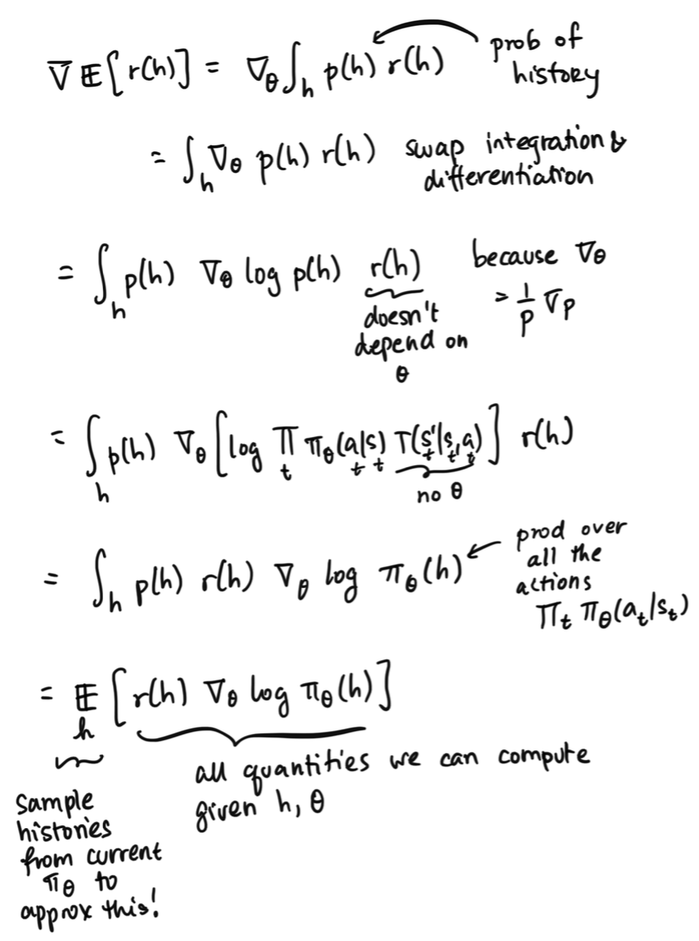
Policy Gradient Derivation
Note: below is just a vanilla example. In real life, you should use Trust Region Policy Optimization (TRPO), Proximal Policy Optimization (PPO), some actor-critic approach.Let $r(h)$ be $\sum_t r_t$ for history h
Let $J(\theta) = E_{\pi_\theta}[r(h)]$ (this is the value, undiscounted, which is what policy gradient folks usually use)
Goal: get $\nabla_\theta J$ so we can update $\theta$ to become $\theta + \alpha \nabla_\theta J$ for $\pi_\theta(s, a)$