Date: April 1, 2020 (Lecture Video, iPad Notes, Concept Check, Class Responses, Solutions)
Relevant Textbook Sections: 9.6
Cube: Unsupervised, Continuous, Probabilistic
Lecture 16 Summary
- Intro: Probabilistic Embeddings
- Variations of Probablistic Embeddings
- Deep Dive into Topic Models Speciifcally
- Quick Detour: Dirichlet Distributions
- Relationship with Other Models
- Continuing with Topic Models: Moving to Inference
Intro: Probabilistic Embeddings
Last time, we looked at PCA as an example of nonprobabilistic embeddings. Today will look at probabilistic embeddings, where we have a probabilistic model for a continuous z that produces an x. One specific type of model within probabilistic embeddings is the topic model. A quick real world example that uses a topic model is the following: there was a study that was done in Pompei where they looked at rooms in the households, marked down the objects they found and their counts, and used a topic model to hypothesize the purpose of the room. Essentially, they'd note down items like doors, chests, cupboards, glass bottles (and their respective counts) etc, which helped indicate what the purpose of a room might be. The reason this is probabilistic is because each room could've had more than one purpose, so we want to capture the fact that a single room might have had multiple purposes, and hence we use a topic model.Variations of Probablistic Embeddings
First, let's look at the variations of probabilistic embeddings (embeddings means unsupervised with continuous z, there's a lot of alternate terminology that means the same thing, such as manifold learning, but we use the term probabilistic embeddings in this course). Later, in the next section, we will jump into a specific example (topic models) within probabilistic embeddings.First, remember our general set up of our z's generating the x's.
Factor Analysis
$$z \sim N(0, \mathbb{1})$$ $$x = Az + \epsilon$$ In factor analysis, we had z drawn from some normal distribution, and x was given by some matrix A times z plus some noise. This is an example of a probabilistic model where we posited that there is some latent k dimensional z that somehow leads the data to become a D dimensional x. The analog in the Pompei example is if we theorized that perhaps a combination of purposes of a given room leads to certain items that are found in the room (which became our x data) in certain counts. Also something to note is specifically, in factor analysis, we are assuming that there's some linear relationship in the mixture of purposes of the room to the counts of items in the room.Variational Autoenconder
$$z \sim N(0, \mathbb{1})$$ $$x = f(z) + \epsilon$$ Now, we have pretty much the same thing, but our f is nonlienar. So it could be the same story from before regarding Pompei, but this time we believe there's some more complex, nonlinear relationship in the mixture of purposes of the room to the counts of items in the room.Deep Dive into Topic Models Speciifcally
We're now going to take a deep dive into topic models specifically. While this is indeed a specific model, many of the concepts and patterns here will be generalizable to other similar models, so keep the big picture in mind when we're working on this topic.Motivation for topic models: suppose we have high dimensional discrete data. For example, codes in a health record. In addition, we believe that these counts of discrete items come form a lower dimensional structure (say, a disease). For example, a disease can lead to many kinds of health codes. You can imagine that a single disease could create diagnoses codes, procedures codes, lab value codes, prescription codes (which are the x's that we see).
Student Question: Why is the above example continuous z? It sounds like z is discrete, referring to the different diseases? That's a great question. So what's important is that we need to remember that we are looking at the patient level. As in here, a single data point is all the medical codes for a single patient. In this story, each patient will have their own z (just like how in clustering, eat data point will have their own z that represented a discrete cluster). But when we actually dig into what our z is in this story, we see that z is going to be continuous and have multidimensional because we are modeling in the fact that the patient could have multiple diseases, and of multiple degrees of severity. For example, for patient Bob, he might have a cardiac disease with 70 percent probability, and a cold with 30 percent probability. In that sense, our z must be continuous.
Another way of thinking about this in another context is looking at the story of restaurants. A given resturant might have a general restaurant food type or perhaps a fuison of food types (z) that affects the menu items (the x data we see).
And to add one more way of thinking, you could think of the context of looking at documents. A given document might have a mixture of document types (the z's) that affect the specific words on the document (and also the counts of words on the document).
Let's Look at the Math
To make our thinking more concrete, we also note here that our model is a mixture of multinomials.Part 1: Parameters for seeing the d items (given you're in mixture k)
$\theta_k \sim Dir(\beta)$ is a D dimensional vector that describes the probability of seeing item d if you are in mixture k.
For example, perhaps we had k=0 represent heart disease and k=1 represent having a cold. $\theta_0$ would tell us the distribution of the codes (the actual x data we should see) given that the person has heart disease underneath the hood (our z), and our $Dir(\beta)$ is representing the distribution of the codes. Then, $\theta_1$ would be the distribution of the codes for if the person just had a cold (which would look quite different from the distribution for $\theta_1$, since having a cold and having a heart disease lead to different symptoms). The whole $\theta$ hence is a D by K matrix of probabilities of seeing item d in mixture k
Part 2: Parameters for your probabilities of being in a mixture k
$\pi_n ~ Dir(\alpha)$ is K dimensional, and tells us the proportions of each $\theta_k$ in data n (as in this tells us the proportion of each topic, or the proportion of each disease to begin with)
The Procedure of How the $x_n$'s are Created
$x_n$ is a count vector of items per data point, which is what we observe. In the Pompei example, it would be like: 3 chairs, 2 chests, 0 spoons, etc. We are going to look into how the procedure of how these are created.First, create the $\theta$'s. For each data point n, we're going to sample $\pi_n \sim Dir(\alpha)$, and then we're going to use our $\pi_n$ to create our data $x_n$. Namely, $x_n \sim Mult(\theta \pi_n, L)$ where L is the total# of codes, menu items, or words, whichever topic you're working on.
Note: when you multiply out $\theta$ (which is D by K) and $\pi$ (K by 1), you will get your probabilities for the items in the x (which is patient specific, or document specific, etc, whichever domain you are in) which is D by 1. So we have all the final probabilities we need for that given patient, and then we enter this in as the parameters of the multinomial, with our $x_n$ generated in that distribution's manner.
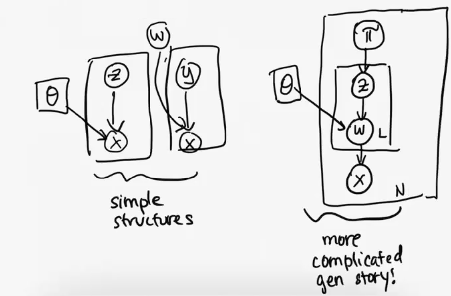
To tie this back into the general setting that we've discussed many times now in our unsupervised learning lectures, where $z_n$ produces the $x_n$ and the w (the global parameters) also affects the $x_n$, here $z_n$ corresponds to our $\pi_n$ and w corresponds to our $\theta$.
Quick Detour: Dirichlet Distributions
We need a process to create $\pi$. Previously, and in the examples given earlier in lectures, we had z distribution as Gaussian. Now, we need specifically the following: $$\pi_{nk} \geq 0$$ $$\pi_{nk} \leq 1$$ $$\sum_k \pi_{nk} = 1$$ We need this to follow these restraints above so that we have probability distribution beacuse then we can interpret it. For example, we want to be able to have the intuition of a restaurant as being mostly Asian cuisine but there's some Latin fusion in it. Or when looking at a patient, we might want to say this patient most likely is a cardiac patient but they also have some chance of diabetes. In the Pompei example, we want to be able to interpret that this room looks like it was used for cooking with this probability, but also rituals with this probability. So that's why we want to use the Dirichlet Distribution. It wouldn't make sense for example, to have a negative number (which is possible if we chose Gaussian) in the latent variable in this case. Dirichlets give us samples from the simplex. $$Dir(\pi | \alpha) \propto \prod^K_{k=1} \pi_k^{\alpha_k - 1}$$ This is similar to the Beta distribution (if k=2, this is exactly the Beta distribution). For intuition on how the distribution look for certain parameters, see the diagrams on the wikipedia page.Relationship with Discrete Mixtures
Let's also recap our thinking on how topic models tie to mixture models and factor analysis.Mixture Models
$$z_n \sim Cat(\pi) \textrm{ where } \pi \textrm{ is a distribution over k mixture classes}$$ $$x_n = \mu_{z_n} + \epsilon$$Topic Models
$$\pi_n \sim Dir(\alpha)$$ $$x_n = Mult(\theta \pi_n, L)$$Factor Analysis
$$z_n \sim N(0, I)$$ $$x_n = Az_n + \epsilon$$Some Comparisons
The idea is in the same way in the mixture models (and factor analysis) where once when we had our $z_n$ we could then determine our $x_n$ (after incorporating our global parameters), in topic models once we have the $\pi_n$ then we can create our $x_n$ (after incorporating our global parameter $\theta$).The difference between mixture models and topic models + factor analysis, is that in topic models and factor analysis, our $\pi$ and z's are continuous, whereas in mixture models, z is still discrete.
The difference between topic models and factor analysis is that we've decided in our topic models that we think the data itself (the x's) is discrete sets of counts, whereas in factor analysis our data is continuous.
Continuing with Topic Models: Moving to Inference
Using the Same Generative Model as Before
Let's now continue on with topic models and move to inference. We can start off by just using the generative model we have as is: $$p(x|\pi, \theta) = \prod_d (\sum_k \pi_k \theta_{kd})^{x_d}$$ Where inside, we have $\sum_k \pi_k \theta_{kd}$ which represents the probability of dimension d, $x_d$ represents the number of times element d was observed, $\sum_k \pi_k \theta_{kd})^{x_d}$ then represents the probability of seeing $x_d$, then finally we take the product over d to have our final probability of x overall. Next, let us take the log: $$\log p(x | \pi, \theta) = \sum_d x_d \log(\sum_k \pi_k \theta_{kd})$$ This is tricky! How can we make this easier to work with? Let's create an equivalent generative model.Using a New Equivalent Generative Model
Globally:$\theta \sim Dir(\beta)$ (for the rest of lecture, let's assume $\theta$ is a parameter)
Locally:
for each n:
----$\pi_n \sim Dir(\alpha)$
----for each l in L_n:
--------$z_{nl} \sim Categ(\pi_n)$
--------$w_{nl} \sim Categ(\theta_{z_{nl}})$
And then: $x_n$ keeps counts of w_{nl}.
The new proposal is I want to geenrate data for a new patient. First I'm going to determine the mixture weights of the different diseases. Just for simplicity's sake, some oracle is going to tell us the patient has this $L_n$ (the number of codes we need to generate for a given patient). Once we know it, then for each given code, we can first ask, what disease are you (the $z_{nl} \sim Cat(\pi_n)$)? Once we pick the disease, then we can then pick the code given that we know what disease is (the $w_{nl} \sim Categ(\theta_{z_{nl}})$) now for this patient (this means we are assuming that these codes are independently drawn).
In story form, if we were doing the restaurant setting where we picked the words on the menu to be what we're counting, we might have something like:
$w_{nl}$ = {of, pizza, of pasta}
We can convert this to an x_n by:
$$pizza: 1$$ $$pasta: 1$$ $$of: 2$$ This is known as the bag of words representation. Also, for reference, below is the diagram for the new graphical model (on the right). On the left are our more simple representations from before, for reference.
Why did we do this?
We did this because in the original set up, it was impossible to solve easily as running the EM algorithm wouldn't work. Even given the $\theta$, it would be hard to find $\pi$, and given $\pi$ it was still hard to find $\theta$. Here, we've introduced a new variable z that let's us do EM (more details on this below). This is apparent if we write out the new likelihood. We now have the following: $$p(x|z, \pi, \theta) = \prod_l \prod_d \theta_{dk}^{\mathbb{1}(w_{nl} = d) \mathbb{1}(z_{nl}=k)}$$ Where $\prod_l$ represents product over all the words in the document, $\prod_d$ represents the product over all the possible word assignments, $\prod_k$ represents the product over all the topics/mixtures, and then we have the $\theta_{dk}$ (probability of a particular dimension occuring) with the indicators that check to make sure we're in the right topic $\mathbb{1}(z_{nl}=k)$ and did we actaully observe the right dimension/word $\mathbb{1}(w_{nl} = d)$. $$log p(x|z, \pi, \theta) = \sum_l \sum_d \sum_K \mathbb{1}(w_{nl} = d) \mathbb{1}(z_{nl}=k)$$ Next, let's get the rest of what we need to do the EM algorithm. $$p(z | \pi) = \prod_k \pi_k^{\mathbb{1}(z = k)}$$ $$p(\pi) = \prod_k \pi^{\alpha_k - 1}$$ $$log(p(x, z, \pi | \theta)) \propto \sum_n [[ \sum_k (\alpha^k - 1 + \sum_l \mathbb{1}(z_{ln} = k)) \log \pi_k] + \sum_d \sum_k (\sum_l \mathbb{1}(w_{ln} = d) \mathbb{1}(z_{ln} = k)) \log \theta_{dk} ]$$ That final term is found by combining the $\log p(\pi)$ term, $\log(p(z | \pi))$ term, and $log(x | z, \pi, \theta)$ term.We note that $\mathbb{1}(w_{ln} = d)$ is known and fixed. This means, for inference: we can run an EM where we take expectations across with respect to z, which will turn those indicators above $\mathbb{1}(z_{ln} = k)$ into $q_{ln}$'s, and then we can maximize with respect to $\theta$, and $\pi$. By rewriting this, we were able to separate out the inference in a way that's nice to do, that let's us apply the EM algorithm!
Note: There are other ways to use this new genreative form to simplify inference: if you can sample z, then you can sample $\theta$, $\pi$ (this content is covered in CS281). You could sample z, and integrate out $\theta$ and $\pi$. The biggest clever part in the graphiacl model was we fixed the z, breaking up the rleationship betwen the $\theta$ and the $\pi$. Before it was interacting in a complicated way, but by having z fixed (since it was sampled), then we can do inference about $\pi$ and $\theta$ separately. This will be discussed and made more formal in the upcoming lecture on graphical models.