Date: April 20, 2021
Lecture Video
iPad Notes
Slides
Lecture 22 Summary
Model-Based Learning
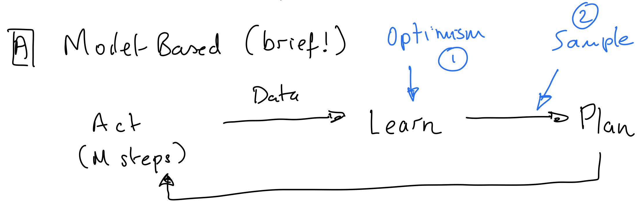
In model-based learning, we cycle through taking actions, using data from those actions to learn a model, using the model to make plan, and then using the plan to continue acting. How do we handle exploring vs. exploiting in this framework? (Recall: in model-free RL last week, we used $\epsilon$-greedy action selection to balance exploration and exploitation.)
Optimism under uncertainty. Let $N(s,a)$ be the number of times we visited the state-action pair $(s,a)$. Each “visit” is a time that the agent was in state $s$ and chose to perform action $a$. When we are learning, we will assume that if $N(s,a)$ is small, then the next state will have high reward. When we do this, we are being optimistic about the state-action pairs we’re uncertain about. Then, we plan using this optimistic model. Since the model thinks taking visiting lesser-known state-action pairs will lead to high reward, we’ll have a tendency to explore these lesser-known areas.
Posterior sampling (Thompson sampling). We maintain a posterior (Dirichlet) on the transition function $p(\cdot | s,a)$. We sample from this posterior to get a model, which we proceed to plan with. The idea is that when we are less certain about the outcome of the transition function, there’s a greater likelihood of the sampling leading us to explore. When we are more certain about what the best outcome is, we’re more likely to just stick with that best outcome.
Back to Model-Free Approaches
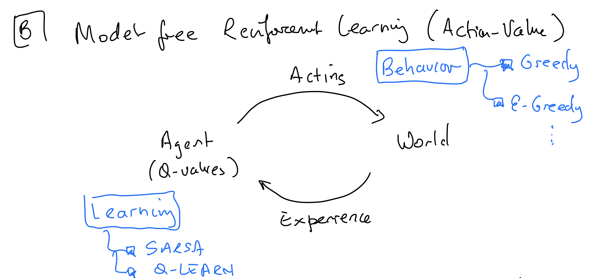
In model-free RL, the cycle is different from model-based RL in that we are no longer learning a model and planning. Instead, feedback from the world is directly used to update the agent. Different Model-Free RL algorithms vary in how the agent selects its behavior (e.g. greedy or $\epsilon$-greedy) and how it learns (e.g. how it updates its Q-values).
Recall from last lecture our discussion on Q-values, SARSA, and Q-learning. We had a definition of the optimal Q-function, which could be used to find the optimal policy. (In each step, the data collected is of the form $s, a, r, s’, a’$: $s$ is the current state, $a$ is the action the agent took, $r$ is the reward received, $s’$ is the next state, and $a’$ is what the current policy recommends for the next action.) $$Q^*(s,a) = r(s,a) + \gamma \sum_{s’}p(s’ | s, a)\max_{a’}Q^*(s’,a’)$$ $$\pi^*(s) \in \arg\max_a Q^*(s,a)$$ SARSA: On policy. Learns Q-values corresponding to the agent’s behavior, so what the agent learns depends on how the agent is behaving $$Q(s,a) \leftarrow Q(s,a) + \alpha_t(s,a)[r + \gamma Q(s’, a’) - Q(s,a)]$$ Q_LEARN: Off policy. Learns Q-values $Q^*$ corresponding to the Bellman equation $$Q(s,a) \leftarrow Q(s,a) + \alpha_t(s,a)[r + \gamma \max_{a’}Q(s’, a’) - Q(s,a)]$$ (For the next part of the lecture, we will require $\alpha_t(s,a) = 0$ unless $(s,a)$ was visited at $t$.)
When certain conditions are satisfied, we actually know for sure that Q_LEARN will converge to $Q^*$. We are not going to prove this theorem, but it comes from Bellman equation and contraction property-esque ideas similar to some of what we discussed last week.
Q-Learning Convergence Theorem
Q_LEARN converges to $Q^*$ as $t \rightarrow \infty$ as long as- $\sum_t \alpha_t(s,a) = \infty$ for all $s,a$. This means we need to visit each $(s,a)$ infinitely often. $\epsilon$-greedy helps with this by ensuring that all the state-action pairs still have a chance of being visited.
- $\sum_t \alpha^2(s,t) < \infty$ for all $s,a$. This can be achieved by reducing the the learning rate; e.g. $\alpha_t(s,a) = \frac{1}{N_t(s,a)}$.
- Behavior is “greedy in the limit”. That is, the behavior eventually follows the Q-values with no exploration. To satisfy this condition, we usually set $\epsilon_t(s) = \frac{1}{N_t(s,a)}$, so $\epsilon$ is decreasing as we visit each state-action pair more often.
Deep Q-Networks
By combining Q-learning with neural networks, researchers have been able to achieve amazing results like learning how to play video games. In an Atari game, each state is comprised of four $84 \times 84$ pixel arrays representing the video game screen at times $t-3, t-2, t-1, t$. One frame can provide information about the current locations of objects in the game, but we need multiple frames to capture attributes like velocity and acceleration. After around 500 iterations of training on the game Breakout, where the player hits a ball upwards to break through a wall of blocks, the RL agent was able to find a clever game strategy that even the engineers working on the project didn’t know about!Representing all of the game states in a table doesn’t work; there’s just too many states. So to parameterize $Q(s, a ; w)$, we use a differentiable deep network with parameters $w$. This network will take in a state and generate predictions for the Q-values of taking each action from this state. In this framework, we are trying to use our gradient descent updates to find a model that minimizes the squared error between the estimated Q-values and the actual Q-value from our experiences in the environment. The TD error, the value we try to minimize, is the $r + \gamma \max_{a’} Q(s’, a’, w_{old}) - Q(s,a, w)$ term we’ve seen in our Q-learning update.
To train the network, we set $$w \leftarrow w - \frac12 \alpha_t \nabla_w[r + \gamma \max_{a’} Q(s’, a’, w_{old}) - Q(s,a, w)]^2 = w + \alpha_t\left (r + \gamma \max_{a’}(s’, a’, w_{old}) - Q(s,a; w)\right )\nabla_w Q(s, a; w)$$ Finally, we introduce experience replay. We put $(s,a,r,s’)$ into a replay buffer, then do mini batch gradient descent steps by sampling sets of memories from the replay buffer. This means we continually reuse our experiences instead of just learning from each experience once.
Policy Learning
Another model-free learning method is policy learning, where we adopt a differentiable policy $\pi_{\theta}(a | s)$ with parameters $\theta$. We’ll learn the policy directly, without any Q-values, models, or planning. This is useful for cases where- There are continuous actions that are impractical to store in a table, such as if we could choose any magnitude of force to apply during an action.
- The policy could be much simpler than the Q-table, making it easier to learn directly. What if we set up a huge Q-table, only to find that the optimal policy is to go right in every state?
- It could be easier to incorporate expert knowledge. Maybe we want to initialize our model with suggestions from an expert (like a human video game player) about what to do. The human player likely has an idea of what a starting policy should look like, but is less likely to have some internal Q-table.
AlphaGo
Go has historically been seen as the hardest game for AI to learn how to play. The game is incredibly complex, with a much larger state and action space than chess. For the rest of class, we’ll discuss how AlphaGo managed to beat a Go champion in 2016. The documentary we watched snippets of in class can be found here, and a full paper about AlphaGo here. For representing the state of a game, the team decided on hand-crafted per-position features to reduce the enormous state size to a $19 \times 19 \times 48$ space, with $48$ features for each position on the $19 \times 19$ board. For training, a combination of supervised learning and reinforcement learning was used.A model $\pi_{SL}$ came from supervised learning, where a deep net was trained to predict expert moves using log likelihood loss. This took three weeks of training on 50 GPUs. Then, the team trained a separate model $\pi_{FAST}$, which was a linear softmax model trained with log likelihood loss and the hand coded features. For the reinforcement learning portion, a neural network was initialized from the $\pi_{SL}$ model. The reward function was +1 for a win, -1 for a loss, and 0 for a draw. The model engaged in self-play games with earlier versions of itself over the course of a day, with updates done using the policy gradient method we discussed earlier. Finally, supervised learning was used to train an estimate of $V_{\theta}$, where the goal was to predict whether the current state would result in a win or a loss. This last part was trained for 1 week on 50 GPUs and 30 million positions.
Using these models together, AlphaGo selected moves using a guided Monte Carlo tree search. This is computationally very expensive, using 48 CPUs, 8 GPUs, and 40 compute threads. Essentially, the agent builds a lookahead tree “looking into” the future, which branches out depending on the actions taken (the actions selected to incorporate in the tree are decided using $\pi_{SL}$ and Q values backed up from leaves). Once a leaf of the tree is reached, $\pi_{FAST}$ and $V_{\theta}$ are used to approximate the value of the leaf state.
Note: $\pi_{\theta}$ wasn’t even used. The team found that $\pi_{SL}$ was more useful.