Date: April 8, 2021 (Concept Check, Solutions)

Lecture Video

iPad Notes

Slides

Concept Check Detailed Notes

Lecture 20 Summary

• Intro: Moving from Predictions to Decisions
• Intro: Markov Decision Processes
• How to Solve using Value Iteration (Method 1)
• Recap and Looking Forward

Intro: Moving from Predictions to Decisions

So far in CS181, we've been looking at how to make predictions. Today, we will transition from predictions into the realm of decision making.

To best illustrate this, let's cover a few real world examples. Imagine we're using a map system to go from a starting point to a destination. The map system might have predictive tools that tell us where the traffic is (using realtime data of where cars are right now), and how long different routes take from start to finish. Modeling was used here to figure out all this traffic information and which routes are slower and faster. But now, we need to make a decision. Which route do we take? We might have different objectives. Maybe we want the route that is the shortest in expectation. Maybe we're okay with being a little slower on average, if there is a guarantee that we'll be there by some time (say we're trying to make an important interview). These are decisions that don't take place at the prediction time. In order to make these decisions, we'll need to formalize a reward function.

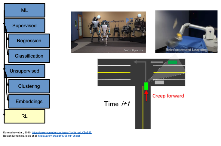
Another real world example is autonomous vehicles. There are tons of predictions that come into place for autonomous vehicles, including where the road is, where the lines on the road are, whether there are signs ahead or not, whether there are pedestrians crossing or not, etc. These are all predictive, and is what we've been doing so far in CS181. Once we have this data, how do we decide what to do next? How should the car drive to be safe? Another example is shown below, where we have a reinforcement learning algorithm that is being used to predict when to creep at a stop sign to position a camera on the vehicle to see if the car is indeed parked or waiting at the stop sign. We also have uses for reinforcement learning in the context of delayed rewards. Alpha Go recently used a method of reinforcement learning, and had to learn strategies despite having rewards delayed far in the future. Those are the types of things we will start looking at across the next three lectures. Let us define a few key concepts about reinforcement learning. Firstly, we have a state. This is something we can observe about the world around us. We then have a decision problem regarding choosing an appropriate action from that state. That action will come with a reward, and the learning problem will be to optimize the choice of actions given states to maximize the reward. One key question remains how to quantify rewards (ie. the reward function), which will guide the learning problem.

Intro: Markov Decision Processes

First: what is a Markov Decision Process? At the most basic level, it is a framework for modeling decision making (again, remember that we've moved from the world of prediction to the world of decision making). In our model, there is only one agent, and this is the agent that needs to make decisions while interacting with the world (other models incorporate multiple agents, but in CS181 we are only covering situations that have one agent).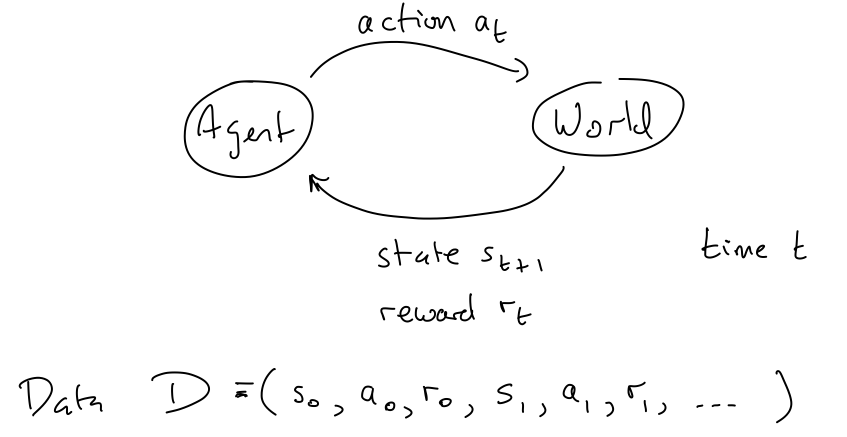

Some Notation, Definitions, and the Goal

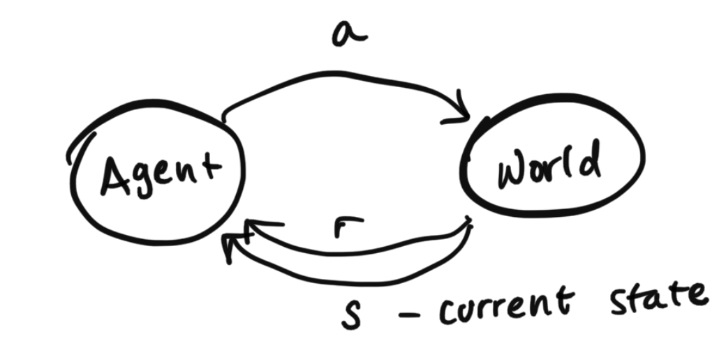
To explain the setup diagram above, the agent can send actions to the world, and the world will return observations that we call $o$ and rewards that we call $r$.

$S = \{1, \dots, |S|\}$ represents the states

$A = \{1, \dots, |A|\}$ represents the actions

$P(s'|s, a)$ defines the transition model

$\pi(a|s)$ is the probability of taking action $a$ given that we are currently in state $s$. This is also known as the policy.

$r$ represents rewards

$t$ represents the time stamp

$\gamma$ is our discount factor which is between [0, 1) (in the future, rewards are worth less by a factor of $\gamma$ per round of time)

Definitions:

Markov Assumption: $P_t(s_{t+1}| s_1, s_2, \dots, s_t, a_1, a_2, \dots, a_t) = P_t(s_{t+1}| s_t, a_t)$

Stationarity assumption: $P_t(S_{t+1} | S_{t}, a_t) = P_t(S_{t+1} | S_{t}, a_t)$. Notice here that we have dropped the subscript $t$, and that the transition model is time invariant. In other words, we can move the time around, and as long as we have the same state $s$ and action $a$, the probability should remain the same.

Types of problems:

The MDPs that we are trying to solve are dependent on the set of variables given by MDP(S, A, r, P), where the state and action spaces are discrete. This means that the transition and reward functions can be more easily computed.

• Planning: the input is an MDP and the output is the optimal policy.
• Reinforcement learning: the input is the access to the world and the outputs are the actions (ie. the policy). This is equivalent to learning from feedback to optimize a policy.

With the above information, we have:

Goal: Agent should choose the actions to maximize the expected sum of discounted rewards. Find the best policy. We use $\pi$ to denote a policy. Policies can be stochastic, or describe a distribution over actions ($\pi(s, a) = P(a|s)$), or determinstic and be equal to 1 action ($\pi(s)=a$). Stochastic policies have a probability distribution across actions for a given state (what probability to play each action with). Deterministic policies we simply have one predetermined action in the policy to play for each given state. These both are commonly used notations.

State: summarizes a history such that making predictions about the future given the state is equivalent to making those same predictions given the entire history.

Breaking Down Definition of State

Imagine we had a situation where we wanted to get a person from Start (S) to Goal (G). Assume we have total control of where our person walks. The solid wiggly line to the middle point is the person's walking history. If the person takes the action, "Go Down", and we try to guess what happens next, we don't actually need to know anything about the history of where the person walked to get to their current location (the middle dot). The person could have taken the solid wiggly line or the dotted wiggly line to get to the middle dot, yet all we really needed to know was their current location. Similarly, if someone stopped you on the street to ask how to get to Maxwell Dworkin, you wouldn't ask them "where did you come from?". You already have enough info to direct them to MD, since you already know their current location. In this example, the person's location is their state, as it is a sufficient statistic.

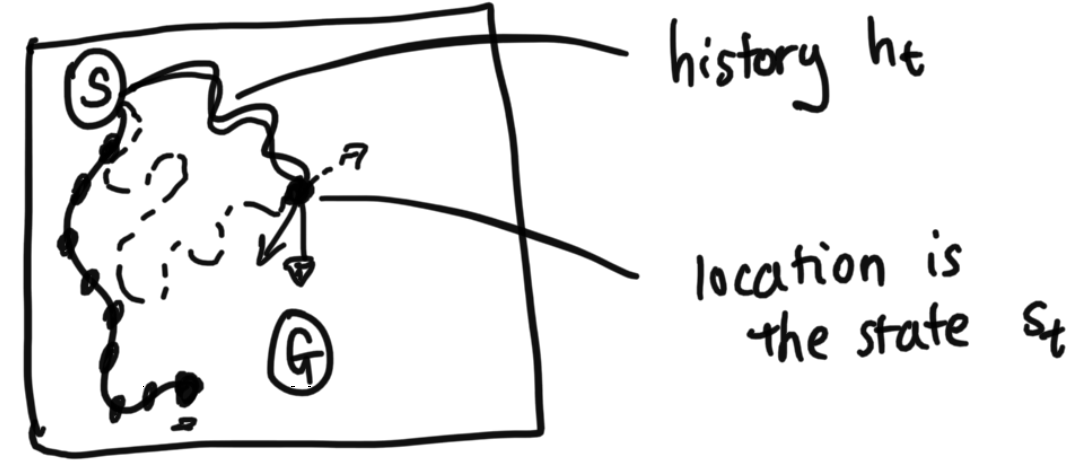
Let's say instead of a person that this was a car instead, however, and that the car's velocity matters. If the car was coming in at 100 miles per hour from the left, moving "Down" would require a huge turn, versus if the car was driving in slowly from above, at 10 miles per hour, the action "Down" would cause the car to move differently in each scenario. This means that only knowing the car's location is not enough to define the car's state. We would want to incorporate in the velocity, the acceleration, and everything we need to be able to predict what happens next. State is all information needed to be able to ignore the past. If all of this information is available to us, then we say the system is Markov in state.

Note: this is the official definition of state. Some papers in the literature will sometimes use approximations of states. Say, for example, you might choose to use a single frame (a still snapshot) of a video game (such as Super Mario Bros) as a state. Therefore from the still frame, you can see where each object (such as Mario, bricks, and evil mushrooms) is located on the screen. But to really predict how the objects move, you actually need the velocity of the objects (is Mario running? in what direction are the mushrooms walking?) to predict what happens next and to be able to call the system Markov. It's possible that the paper will just say, "We will choose to use just the frame as our approximation of state". It's just important to note that that is exactly what it is: an approximation of a state. However, the formal definition of state is still everything you need to know to be able to predict what's next. We will use this definition for state for the next 3 lectures.

Tying Back and Fully Defining our Markov Decision Process

Let's come back to the diagram of an agent in the world. Now, we're going to assume the world is nice, and that when our agent does some action $a$ from starting state $s$, the world will send back the resultant state $s'$. You can imagine that the obsevations we had from the situation before get converted via some method into the state (in the real world, this is what would have to happen). Because the world gives us a resultant state $s'$ which gives us all information we need to predict what will happen to the agent next, this system is a Markov Decision Process.

Now let's fully define everything:

This system can be described using this tuple of information: $$\{S, A, R(s, a, s'), T(s' | s, a), \gamma, p_0\}$$ $S$ are all possible states
$A$ are all possible actions
$R(s, a, s')$ is the reward for doing action $a$ in starting state $s$ and landing in state $s'$
$T(s' | s, a)$ is a matrix of transition probabilities, which describe $p(s' | s, a)$, the probability of landing in state $s'$ from taking action $a$ from starting state $s$. Notice this is a similar idea to the last time when we were defined T(s'|s) for Hidden Markov Models. The only difference is that here, transition probabilities depend on the action.
$\gamma$ is the discount factor. $p_0$ is some starting state.

Objective:

• Infinite Horizon: $max_{\pi} E_{T, p_0}\left[\sum_{t=0}^\infty \gamma^t r_t \right]$. Our goal here is to find the policy $\pi$ that maximizes the expected value of this expression.
• Finite Horizon: $max_\pi E_{T, p_0} \left[ \sum_{t=0}^T r_t \right]$ With a finite time horizon, we do not need to discount (although we may choose to), but we are still trying to maximize expected reward from the policy. For an infinite time horizon, we needed to discount to have convergence of our expectation.

Here, $T$ and $p_0$ represent transition probabilities and the initial starting state of the world. The agent does not have control over the world. The agent does control its own actions. We are trying to determine the best actions for the agent to take: the actions that maximize the agent's rewards that it gets in the world.

How to Solve using Value Iteration

Over the this lecture and next, we will cover three methods of solving an MDP. Each will have their pros and cons. There's a lot of literature on this topic that includes more complex methods, but overall the three we cover are intuitive and scale relatively well. Additionally, the complex methods build off these simpler methods here, so this is laying down important groundwork.

First, let's explore value iteration. At a high level, value iteration is similiar to dynamic programming in that it evaluates the optimal actions based on the best values it can achieve in a future time step. We will evaluate value iteration in the context of the finite and infinite time horizons.

Finite Horizon Planning, Value Iteration

Define $V^*_{(t)} (s)$ as the total value from state $s$ under optimal policy with $t$ steps to go. Notice that in this notation, $t$ counts the $\textit{remaining}$ steps, and does not count the current time step. As such, iterating to the next time step will decrease the index $t$ to $t-1$. Taking a page from dynamic programming, we can derive a principle of optimality to work backward from the last time step. The principle of optimality states that:

An optimal policy consists of:
• An optimal first action
• Followed by an optimal policy from the successive state

This brings us to the algorithm for value iteration

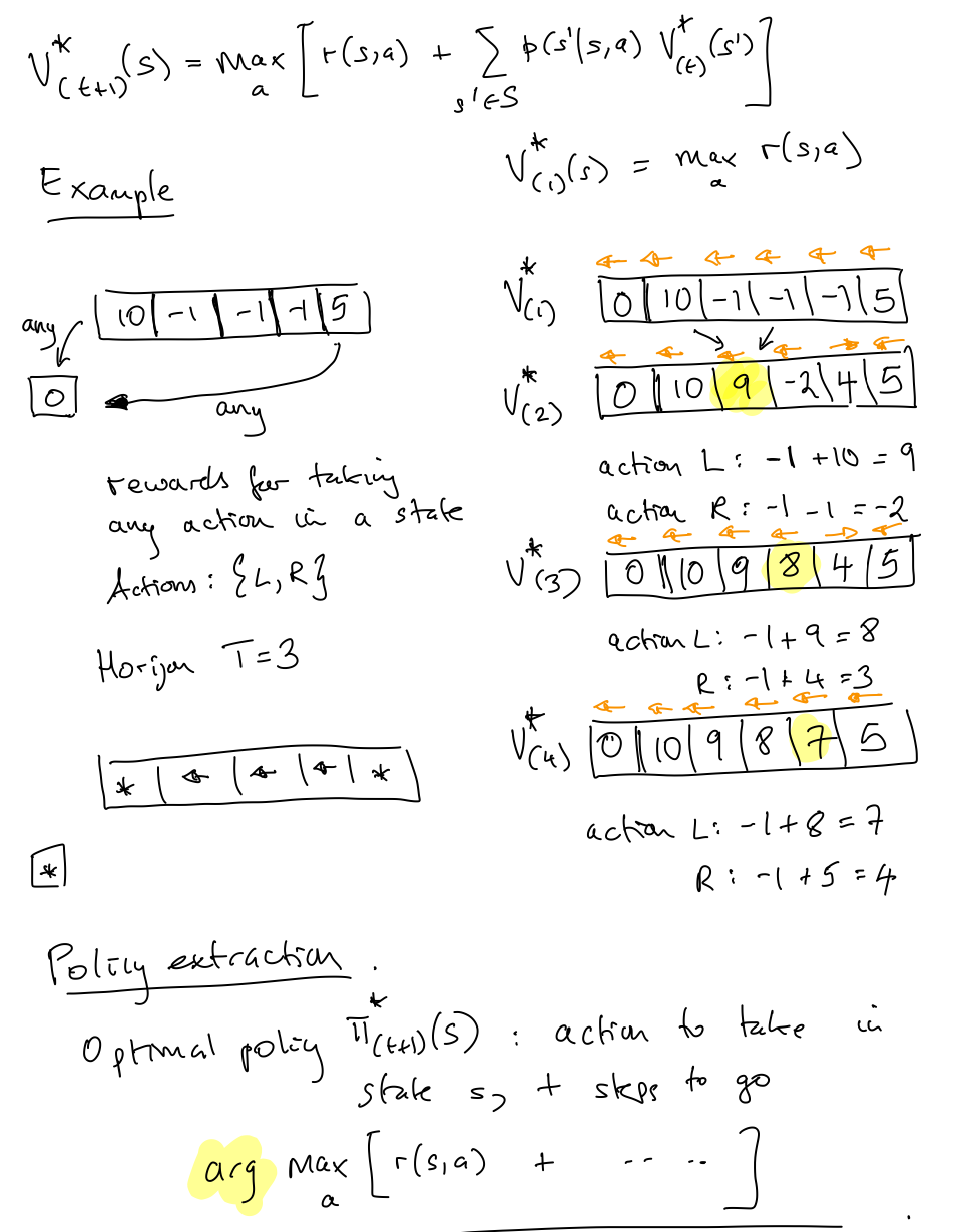
• Base case: $V^*_{(1)(s)} = max_a r(s,a)$
• Inductive case: $V^*_{(t+1)}(s) = max_{a}\left[ r(s,a) + \sum_{s'\in S} p(s'|s,a) V^*_{(t)}(s')\right]$. Notice that we have already calculated $V^*_{(t)}(s')$, which is similar to how we might think about dynamic programming. $s'$ is the very next state.

Example from class: In this example, we have an absorbing state after leaving states with reward 10 or 5. At each state (other than the states at the ends of the line), there are two possible actions. The goal here is to find the maximum value we can extract with $t$ time steps remaining, as well as the corresponding policy with that time step. Notice that for $V^*_{(1)}$, our policy for each state is limited by the fact that we only have one move remaining. As such, the value is just the reward at that particular state. However, as we consider $V^*_{(2)}$, there are a set of possible states to which we can transition, and each of those states has a corresponding reward. For instance, the second state, which had a maximum value of -1 for $V^*_{(1)}$ now has a maximum value of 9. This is because the agent can now select the action to move left, and therefore receives the reward at the current state and the reward of 10 at the next state, which is the optimal value given that we have two moves. We can therefore perform policy extraction to derive the optimal policy for the remaining number of time steps by finding the action set at each state that maximizes the value.

The computational complexity of value iteration is $O(T |S| |A| L)$, where $L$ is defined as the maximum number of states reachable from any states through any action.

Infinite Time Horizon, Value Iteration:

Assume a deterministic policy, $\pi(s) \in A$. We then define an MDP value function: $$ V^{\pi}(s) = E_{s \sim p} \left[ \sum_{t=0}^\infty \gamma^t r(s_t, \pi(s_k)) | s_0 = s\right]$$ In words, this essentially refers to the expected discounted value from policy $\pi$ in state $s$. $$V^{\pi}(s) = r(s, \pi(s)) + \gamma \sum_{s' \in S} p(s'|s, \pi(s)) V^{\pi}(s'))$$ We define the optimal policy to be: $$\pi^* \in arg max_{pi} V^{\pi}(s)$$ for all possible states. The optimal value function is defined to be: $$V^*(s) = V^{\pi^*}(s)$$ We will continue to expand on solving this through the Bellman equation next week.

Recap and Looking Forward

Where are we so far? So far, we've found one way of getting the optimal policy. We will cover two more methods in the next lecture. In addition, soon we will be covering reinforcement learning (RL). RL is learning when we don't have access to $T$, and $R$. What if we had to just interact with the world directly? Much more to come!