Date: April 6, 2021 (Concept Check, Class Responses, Solutions)
Relevant Textbook Sections: 10
Lecture Video
iPad Notes
Lecture 19 Summary
- Fairness and Inequity
- Time Series and Hidden Markov Models
- Questions We'd Like To Answer
- Solving Questions in Collection 1
- Solving Questions in Collection 2
Fairness and Inequity
Fairness and inequity can become extremely complicated in real-world machine learning settings. Imagine a setting where we are determining which applicants will receive a loan from a bank. What if using an ML model makes everyone better off than compared to the old, manual, system, but for some people (maybe demographics with more complete data, people whose financial histories are easier to model, etc.), the improvement is greater compared to other people.Is this fair? In particular, if we optimize a business model like the bank’s for optimizing profit compared to optimizing fairness (one way to measure this is the true positive rate between different populations), the model comes out differently. This means that there are settings where agencies are trading off between fairness and profit.
We’ve only scraped the surface of how nuanced this problem can be. If you’re interested, there’s a great article about fairness in a loan-granting setting here.
Time Series and Hidden Markov Models
Today, we will be covering Hidden Markov Models, a specific Bayesian Network form for studying time series. The idea is that we’re observing something that changes over time. We have an evolving latent state $z$, where $z_t$ is the value of the state at time t. The time goes from 0 to T, the last timestep we measure at.For today, z will be a discrete variable that can take one of $K$ different possible values. We don’t know the true values for what the z’s are, but each $z_t$ produces some measurement $x_t$ that we can observe.
Examples:
- A patient is ill and has true disease states (the z’s) which evolve over time. We don’t know exactly what the true disease state is, but we can observe biometrics (the x’s) like body temperature, heart rate, or presence of symptoms.
- Someone is speaking words (the z’s) and says different words at different times. The computer doesn’t know exactly what words they said, but has the audio signals (the x’s) from a recording of the speaker.
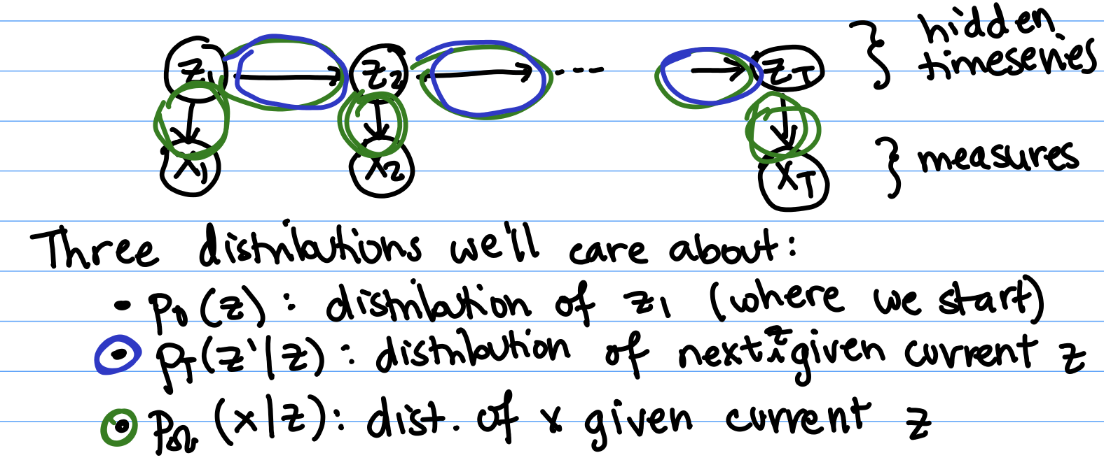
Three Main Global Unknowns/Parameters
Just like in the other settings we’ve studied these past few weeks, Hidden Markov Models have both global unknowns and local unknowns that we might want to infer.There are three main global unknowns or parameters.
- $p_0(z)$: The prior. Which state do we start in? To get our first state $z_1$, we have a prior at 0, which is a probability breakdown describing how likely we are to start off in each of the k states. For example, we know there are certain words that are more likely to be the first word in a sentence.
- $p_T(z’ | z)$: The transition probabilities. This is the probability of our next state being z’ if the current state is z. For example, if the current word is “the”, then the next word is more likely to be “computer” than it is to be “the” again.
- $p_{\Omega}(x | z)$: The observation probabilities given states. Given a latent state z, this tells us the probabilities for what the observation x will be. Example: the distribution of what a robot’s light sensor senses (x) might vary depending on if it’s in a bright, open space vs. a dark, narrow hallway, but each time it’s in a dark, narrow hallway (z = dark, narrow hallway) the sensor distribution will be the same.
Local Unknowns
We also have local unknowns: for every sequence $x_1, x_2 ... x_T$, we do not know the latent states $z_1, z_2 ... z_T$.Questions We'd Like To Answer
Collection 1: Given Globals, Solve for Locals
Given the $p_0$, $T$, and $\Omega$, we want to be able to find out things about z and x. Some specific values we might want to find are:- Filtering: $p(z_t|x_1, …, x_t)$. This is real time prediction. We can only use the data we have so far from observations before time t to make a prediction about time t. Say x’s are radar measurements and z is the potential location of a missile. We want to use the data we’ve seen so far to estimate where the missile might be right now.
- Smoothing: $p(z_t | x_1, …, x_T)$. This is afterward inference. We can use data from before and after time t to make a prediction about t. Say we’ve collected audio from a nature preserve, and we want to use all the information we have from before time t and after time t to determine if a particular bird was singing at time t.
- Probability of Sequence: $p(x1 ... x_T)$. This is the probability that a particular sequence occurred. Perhaps we want to detect outliers in audio, to determine whether a section of the recording was just background noise. We can use the probability of the sequence as a way to tell if it is an outlier or not. Sequence probabilities are also useful for model selection.
- Best Path: $\arg\max_z p(z_1 ... z_T|x_1 ... x_T)$. Finding the best latents. Imagine we have audio of someone speaking, and we want to know the most probable set of words they’ve spoken (z’s) that would produce the data in the recording (the x’s).
- Predict measurements: $p(x_t | x_1 ... x_{t-1})$. We can also try to predict the next observation x, instead of predicting the latent z like we have in most of the previous points. Example: we may want to predict the hospital utilization rate tomorrow given what has happened so far.
Collection 2: Given x's, Solve for Globals
We also want to learn the globals given the x's. Specifically:Given ${(x_1 ... x_T)}$, find the ML or MAP of $p_0$, $T$, $\Omega$
This is important because we need to learn some value for the globals before we are able to do the problems in collection 1. The full joint probability of seeing a particular set of x’s and z’s in an HMM is $$p(x_1,…,x_T,z_1,…,z_T) = p_0(z_1)\prod_{t=1}^{T-1} \underbrace{p_T(z_{t+1} | z_t)}_{A} \prod_{t=1}^{T} \underbrace{p_{\Omega}(x_t | z_t)}_{B}$$ Where A represents the terms from all the transition probabilities, which describe the probabilities of the $z_t$’s being the values we observed given each $z_t$’s ancestor state $z_{t-1}$, and B represents the terms from all of the observation probabilities, which describe the probabilities of the $x_t$’s being the values we observed given the $z_t$’s.
Note that we can evaluate $p(z_1…z_T | x_1…x_T)$ up to a constant factor just by looking at this joint probability. However, if we wanted something like $p(z_t | x_1…x_T)$, one of the values used in our inference problems above, then we need to marginalize out all of the z’s at other times.
The Forward-Backward Algorithm (FBA) does this efficiently. It’s a special case of the inference methods we covered last week.
Note: FBA is analogous to Kalman filters used for continuous problems. Today, we are assuming the z’s are discrete, but if we generalized to the case for continuous z’s, we’d have a Kalman filter.
Solving Questions in Collection 1
As a recap, collection 1 refers to solving the problems listed from before when $p_0$, $T$, $\Omega$ are known.Forward-Backward Algorithm
In order to solve the questions in Collection 1, we are going to use the forward-backward algorithm from last class. The Forward-Backward algorithm is a special case of last class’s algorithm for this specific time series structure. You can think of this either as a review of last class to make sure we really get it, or as a deep dive into a particular scenario.As we go through the algorithm, we will notice some interesting properties about the math we do. Specifically, at a conceptual level, we'll see later how we essentially have these $\alpha$ terms that are "messages" that feed information forward, and these $\beta$ terms that are "messages" that feed information backward (hence the name). Let's dive into the math. We’ll make a few observations about values we can calculate, then tie together patterns that emerge from these observations.
Looking at $p(z_1)$
$p(z_1)$, also known as $p_0$, is a probability distribution for what state $z_1$ we will start in. This is given to us as the global parameter, and it is a vector with K elements.Looking at $p(x_1)$
The probability $p(x_1)$ (the probability that the first observation will be a certain fixed value $x_1$) can be found by expanding over all possible values for $z_1$. $$p(x_1) = \sum_{z_1} p_0 p_{\Omega}(x_1|z_1)$$ We can think of this sum as the sum of all K entries in the vector V, where V is the element-wise vector product of two K-dimensional vectors: one where the kth entry represents $p(z_1 = k)$ (which is $p_0$), and one where the kth entry represents $p(x_1 = x_1 | z_1 = k)$. (We use “$z_1 = k$” to refer to the case where the true value of $z_1$ is state k of the K possible states.)In this expression, we only incorporate $x_1$ and $z_1$; we’ve ignored all of the other x’s and z’s that may be in the graphical model. This comes from from last week’s result, where we saw how we can prune out a bunch of variables to simplify our probability expressions. All we need to consider are the ancestors of our query and evidence variables, which means we only need to consider $x_1$ and $z_1$.
(When we take $p(x_1)$, $x_1$ is our query variable. $z_1$ is included because it’s the ancestor of $x_1$. Since we’re not conditioning on anything, there is no evidence variable.)
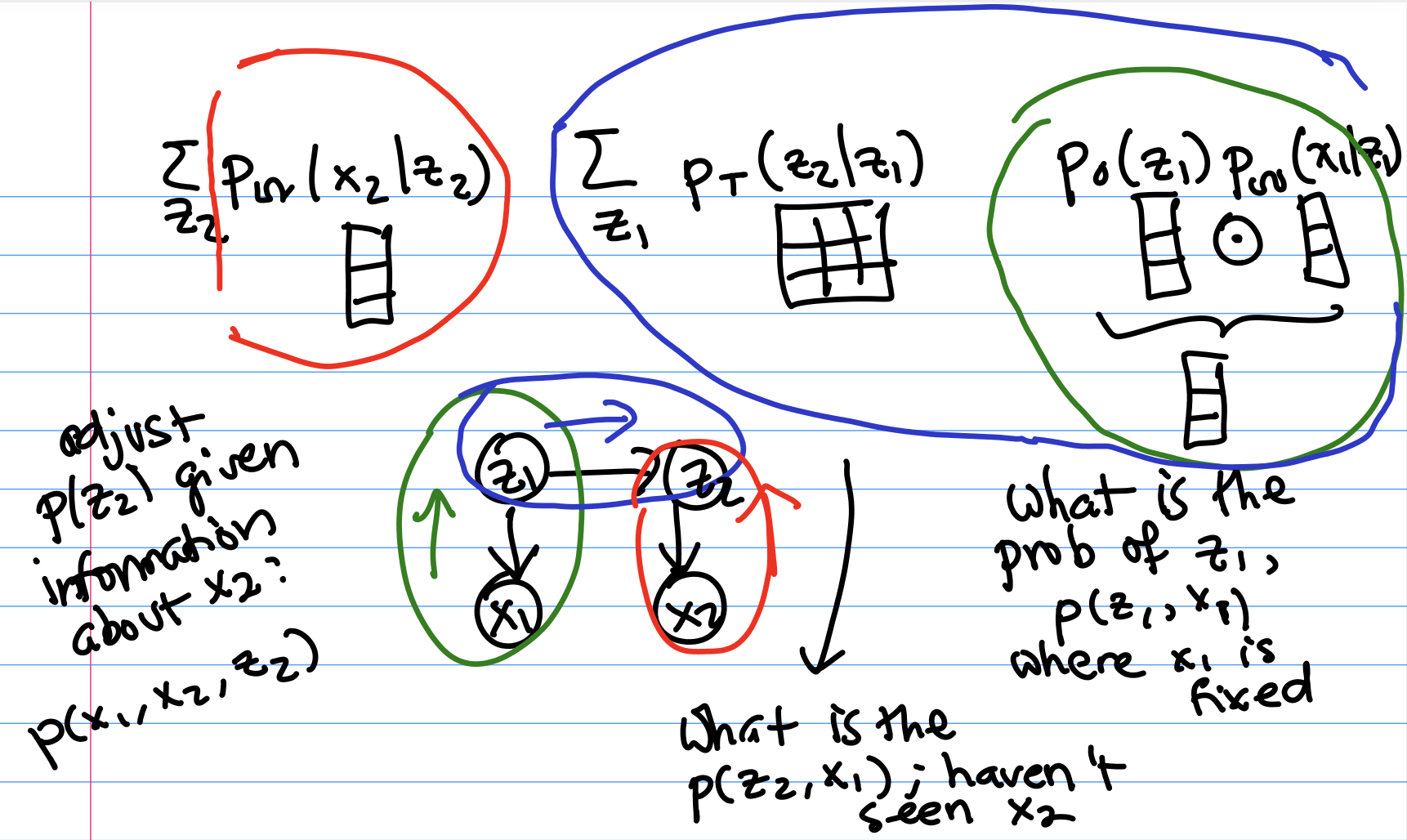
Looking at $p(x_2 | x_1)$
Now, let’s find $p(x_2 | x_1)$. This would be a value used in the Prediction problem mentioned earlier, but we’ll see that calculating it will help us solve all the other problems as well.We know that $p(x_2 | x_1) \propto p(x_2, x_1)$. As before, we only incorporate ancestors, which here are $s_1$ and $s_2$.
$$p(x_2, x_1) = \sum_{z_1} \sum_{z_2} p_0(z_1) p_T(z_2 | z_1) p_{\Omega}(x_1 | z_1) p_{\Omega}(x_2 | z_2) $$ We're going to reorder summations using what we learned in last class. $$= \sum_{z_2} p_{\Omega}(x_2 | z_2) \sum_{z_1} p_T(z_2 | z_1) p_{\Omega}(x_1 | z_1)p_0(z_1) $$ We can think of these two sum terms as incorporating different pieces of information about what $x_2$ might be. In the diagram below, the colors match up portions of the joint probability expression with the associated section of the graphical model. The $\sum_{z_2} p_{\Omega}(x_2 | z_2)$ describes how the value of $z_2$ affects what $x_2$ will be (red). The $\sum_{z_1} p_T(z_2 | z_1) p_{\Omega}(x_1 | z_1)p_0(z_1)$ accounts for how $x_1$ affects our estimate of what $z_1$ was (green), and how $z_1$’s value affects what we think $z_2$ was (through the transition matrix; blue).
If we glue together these two pieces of information, we get our joint probability $p(x_2, x_1)$.
Extending this Method to Arbitrary t
Let's extend the above method to arbitrary time step t. To do this, we will formally define our $\alpha$'s and $\beta$'s, which relate closely to the math we just did above.Defining Alpha
First, $\alpha_t$ is essentially $p(z_t, x_1...x_t)$, in terms of what it captures from the graphical model. It is a K-dimensional vector where the kth entry corresponds to the case where $z_t$ is state $k$. Below is first our base case using the prior, then the general case:
$\alpha_1(z_1)$ = $p_0(z_1)p_{\Omega}(x_1 | z_1)$
$\alpha_t(z_1) = [\sum_{z’} \alpha_{t-1}(z’) p_T(z_t|z’)][p_{\Omega}(x_t | z_t)]$
Note: $\alpha$ is a size K vector. The above equation shows how to calculate the value of one state, but really this needs to be done for each possible state and then combined into a vector. Observe how the math here mirrors the expressions we saw earlier. Here, the $z’$’s refer to possible values for what $z_{t-1}$ is.
To explain the intuition of the math, with regards to the left term, $\sum_{z’} \alpha_{t-1}(z’) p_T(z_t|z’)$, we're essentially getting the previous alpha, $\alpha_{t-1}(z’)$, then accounting for the transition probability to get to the current state. This corresponds perfectly to our specific example from before, where we're incorporating information from the past by using the transition probabilities.
Then, the other term that's part of $\alpha$ is $p_{\Omega}(x_t | s)$, which incorporates information about our current observation. Again, this is the same as in our specific example above.
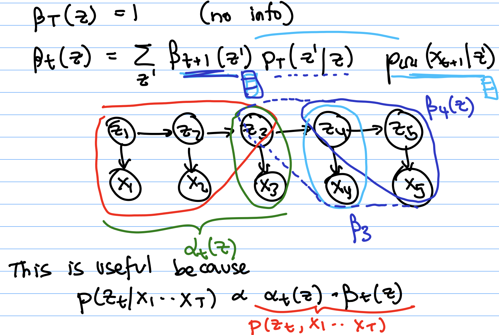
The $\alpha$s can be used to filter for the current state and and make predictions about future observations. But for the problems incorporating the full sequence rather than just previous events, we also need a backwards pass to help us incorporate information from the future. This will be represented by our $\beta$s. It will be just like the $\alpha$s, but in reverse.
Defining Beta
$\beta_t$ is a very similar idea to $\alpha$ but about using information from the future instead of the past. Specifically, $\beta_t$ is the joint probability of future observations, conditioned on the state at $t$. $$\beta_t(z_t) = p(x_{t+1},..,.x_T | z_t)$$ Below, we define a recursive expression for $\beta$.
$\beta_T(z_T) = 1$ (no information when $t = T$)
$\beta_t(z_t) = \sum_{z’} \beta_{t+1}(z’)p_T(z’|z_t)p_{\Omega}(x_{t+1} | z’)$ (only when $t \neq T$)
$\beta_{t+1}$ is info from future. Now for the $\beta$ expressions, $z’$ refers to possible values for $z_{t+1}$. $p_T(z’ | z_t)$ is telling us where we might be now (observe that we’re using the transition probabilities backwards with respect to what we did for the $\alpha$’s). $p_{\Omega}(x_{t+1} | z’)$ is the next observation. We're considering t+1 in the $\Omega$ now, not t, since we are now looking at state values for the future instead of the past.
Example: if the dark blue in the diagram below is $\beta_4$, then to get $\beta_3$ from that, we need to incorporate the information from observation $x_4$ and what it tells us about $z_4$, which is the $P_{\Omega}$. We also need to consider the probability that two particular $z$’s would come consecutively, which is where we use $p_T$.
FBA, the $\alpha$’s, and the $\beta$’s are reviewed in more depth in Textbook section 10.4.1.
Wrapping up: Solving Questions in Collection 1
Now, which of the problems mentioned earlier do we know how to solve?Filtering can be solved with $\alpha$’s: $$p(z_t | x_1,…,x_t) \propto p(z_t,x_1,…,x_t) = \alpha_t(z_t)$$ Smoothing can be solved with $\alpha$’s and $\beta$’s (we break the probability down using what we know about independence in the time series graphical model): $$p(z_t | x_1,…,x_T) \propto p(z_t,x_1,…,x_T) = p(x_1,…,x_t,z_t)p(x_{t+1},…,x_T|z_t) = \alpha_t(z_t)\beta_t(z_t)$$ The sequence and prediction problems can be solved by summing over the $\alpha$’s - see Textbook 10.4.2 for details.
Viterbi Algorithm for Best Path Problem
The only problem we haven’t covered is the best path problem, which we’ll touch on now. The best path problem is the one where we look for $\max p(z_1…z_T | x1…x_T)$. This can be done using the Viterbi algorithm, a dynamic programming algorithm. We will not go through this in great detail, but just sketch out the main idea.First, we recursively define a function $\gamma$ as follows, with two cases depending on whether $t=1$ or not: $$\gamma_1(z_1) = p_0(z_1)p_{\Omega}(x_1|z_1) $$ $$\gamma_t(z_t) = \underbrace{\left[\max_{z_{t-1}} \gamma_{t-1} p_T(z_t | z_{t-1}) \right]}_{\text{best path to } z_t} p_{\Omega}(x_2 | z_2)$$ After finding all the $\gamma$’s, choose each state $z^*_t$ in the optimal path based on the highest $\gamma_t(z_t)$. Start with $z^*_T$ and work backwards. (We will end up needing all $T \times K$ possible values of gamma for different combinations of timesteps and state values, because we take the max over K $\gamma$'s at once in the next step.) $$z^*_t = \arg\max_{z_t} \gamma_t(z_t)p_T(z^*_{t+1} | z_t) $$ Each $\gamma_t(z_t)$ refers to a likelihood for the most probable path for getting to $z_t$. $z^*_{t+1}$ will already be fixed because we are working backwards, so $p_T(z^*_{t+1} | z_t)$ is like also incorporating information about the likelihood of going from $z_t$ to $z^*_{t+1}$.
Solving Questions in Collection 2
Next, briefly, we consider how to find $p_0$, $T$, $\Omega$.First, we note that if we had z, then solving maximum likelihood of $p_0$, $T$, $\Omega$ would be easy. We would just get the empirical distribution over $z_0$'s to get $p_0$. For each z, we could count how often each z’ happens to get the transition matrix. Essentially, we can collect best guesses for the globals we need by just gathering data.
In addition, the process from above tells us how forward-backward algorithm allows us to get z given the globals.
Combining these two ideas, we see that we can apply block coordinate ascent (the same thing we've gone over many times over the last few weeks) to iteratively solve for the global and local unknowns.