Lecture 1 Recap - Nonparametric Regression

Date: January 26, 2021

Relevant Textbook Sections: 2.1-2.2.1

Cube: Supervised, Discrete or Continuous, Nonprobabilistic

Lecture Recaps

Welcome to CS 181! The teaching staff will be writing "Lecture Recaps" for each lecture. The purpose of these lecture recaps is to serve as a resource and reference for you when you wish to review or revisit material as taught in class. These lecture recaps are not scribes, and their focus will be on mathematical content.

Course Introduction

Machine learning is everywhere: with machine learning, we can build some really important and exciting things. In CS 181 we take a critical approach to machine learning: it's not just all about "move fast and break things". There are many examples where algorithms have perpetuated societal biases against people with marginalized identities, including racial and gender minorities. Rigor, professionalism, ethics, and inclusion are essential to our work.

We're going to begin the course with a short discussion about Deepfake videos. Before we get too technical, we're going to think through potential societal implications of the ML. This is an example of a video that very convincingly looks like Obama, but was created using ML:

Some questions one might consider are:

How might you detect a Deepfake video? Were there characteristics of either video that were give-aways that it wasn't real?
Under what conditions might you have issues with these Deepfake videos? What are the ethical concerns?

Generative adversarial networks are used to create Deepfakes. It's somewhat of a "race" against folks detecting Deepfakes, who find ways to distinguish or identify them, and the Deepfake designers who specifically improve their algorithms to address these use cases.

There's other forms of impersionation and manipulation too, that are enabled by technology. But impersonation in itself is not a new phenomenon: photos and media have been faked for years. What is it that makes Deepfakes so concerning? There's been a large amount of media about Deepfakes as a political problem. But one of the most pressing and popular uses of Deepfakes is in revenge porn. A lot of the social consequences are not necessarily political, but deeply interpersonal, shaping the fabric of our relationships.

So how do we make machine learning models? Much of machine learning is about perfecting the "zen", or gaining the wisdom through experience to:

Make appropriate modeling choices
Have sufficient understanding to be able to apply new techniques
Anticipate and identify potential sources of error
Evaluate carefully

Yet to get there, we also need to do a lot of "push-ups". By doing math and deriving popular methods, we'll develop a better understanding of ML.

ML Taxonomy

In CS 181, the methods we study can be split into 3 groups: supervised, unsupervised, and reinforcement learning.

Supervised learning

Supervised learning is defined by using labels $y$ during training. At run-time, an ML model is given a new input $x$, and predicts a label $y$.

There's two variations of supervised learning:

Regression, where labels $y$ are continuous and numeric, or real numbers. Example: Virtu Financial uses regression to predict a stock's future price.
Classification, where labels $y$ are discrete and categorical. Example: "Swipe typing" uses a language model to predict which word is intended from one's typing.

Unsupervised learning

The crucial difference between unsupervised and supervised learning is that in unsupervised learning, there are no labels $y$ available when training. All that is available is data $x$.

Two types of unsupervised learning we'll discuss in-depth are clustering and embedding. Clustering is used to find natural groupings of examples in the data; one popular example is Google News, which delivers groupings of stories about the same topic. Embedding techniques are used to embed a high-dimensional dataset in a low-dimensional space. One example of an embedding technique is point-of-sales data from supermarkets. If we look at time-series data of 1073 products in different locations, and embed the time-series into a lower-dimensional space using a technique called Principal Components Analysis, one of the components actually clearly illustrates the economic effect of the 2008 financial crisis.

Reinforcement learning

In Reinforcement Learning, the data is a sequence of triples: states, actions, and rewards. If a robot is rolling around Cambridge, its state is its current location, the action is which way it moves, and the reward it gets is based on what happens to it after it takes the action (for example, whether it falls into a grate or accomplishes its goal).

Non-Parametric Regression

In this course, we use "The Cube" as a framework to organize the different types of methods we learn. Today, we'll be discussing non-parametric regression, which is a form of supervised learning. Recall that in supervised learning, our objective is to predict labels $y$ from data $x$, where labels $y$ are available to us at training time. We are interested in regression, where labels $y$ are continuous. Non-parametric regression is not probabilistic.

So how do we solve a regression problem? Let's draw a 1-dimensional example:

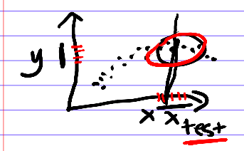
Given some value $x_{test}$, our goal is to predict its corresponding label $y_{test}$.

The first method we'll present, K-nearest-neighbors, is one of the simplest ways to imagine predicting the labels. The intuition is: why don't we just look around the other available data points we have that have $x$-values near our $x_{test}$? Their $y$-values are good $y$-values to propose. To make a prediction for point $x_{test}$, look at the points near the current point, and make a prediction based on them. This is a non-parametric method because its run-time scales with the size of the dataset.

K-nearest-neighbors (KNN):

KNN is one algorithm used for non-parametric regression. Our dataset $\mathcal{D}$ consists of $N$ pairs of inputs and outputs:

$$\mathcal{D} =\{ (x_0, y_0), (x_1, y_1), ... (x_N, y_N)\}$$ Our regression algorithm makes predictions $\hat{y}(x)$ for some input $x$ as follows:

Find the $K$ data points $(x_i, y_i)$ that are closest to $x$.
Predict $\hat{y}(x) = \frac{1}{K} \sum_{k = 1}^{K} y_k$, where the $y_k$ are the corresponding labels for the the are the $K$ nearest $x_k$s to our $x$.

Pros of KNN:

It's flexible! We made no assumptions on the shape of our data, or the relationship between $x$ and $y$.

Cons of KNN:

We need to keep the training data around in order to make predictions. If you have a really big training dataset that has thousands (or millions!) of points, then running KNN may be inefficient and expensive at test-time. Every time you need to make a prediction for some new point $x$, you need to find $x$'s nearest neighbors. (Sidenote: There have been some advances in algorithms and systems that can make these searches more efficient, but this is still a compelling consideration.)
To use KNN we must define "what is near"? For example, say that data $x$ is high-dimensional and complex, like a patient's entire medical record. How can you tell when two patients are similar to each other, given their medical data? The answer isn't obvious.

Kernelized Regression

Kernelized regression is another form of non-parametric regression. To predict label $\hat{y}(x)$ for a data point $x$ using dataset $\{(x_n, y_n)\}_{n = 1}^N$ of $N$ examples,

$$ \hat{y}(x) = \frac{\sum_{n = 1}^{N} K(x, x_n) y_n}{\sum_n K(x, x_n)}$$ The "kernel" or "similarity" function $K(x, x_n)$ outputs a real number that is large when $x$ is "similar" to $x_n$, and small when $x$ is "far" from $x_n$. Note that kernel regression sums over all of the points in the dataset; while KNN only sums over the $K$ nearest neighbors.

Later in the semester, we'll discuss other kernel functions, and properties that determine a valid kernel function. One example kernel function is:

$$ K(x, x') = \exp \left( - (x - x') W (x - x')^T\right) $$ where $W$ is a matrix: one example choice of $W$ could be the identity matrix $I$.

Conceptual question 1: What is the role of the denominator in kernel regression? Can the output of the kernel regressor be a value larger than the maximum $y$-value $y_{max}$ of the training data? Can we get values smaller than the maximum $y$-value $y_{min}$ of the training data?

Answer: The denominator acts as a "normalizing constant". No, we can't get values outside the max-min range of the training data.

Conceptual question 2: Say that we wish to use a non-parametric regressor to make a prediction for an "out-of-distribution" data point, or a data point is far away from the available training data points. What will our regressor do?

This site is out of date.

CS 181