Date: March 30, 2021 (Concept Check, Class Responses, Solutions)

Relevant Textbook Sections: 8

Cube: Probabilistic

Lecture Video

iPad Notes

Lecture 17 Summary

• Intro: Motivation Behind Graphical Models
• Graphical Models
• Bayesian Networks
• Uniqueness and Parameters
• Beyond Bayes Nets

Intro: Motivation Behind Graphical Models

Today we're going to be moving beyond the cube. Just as we moved into more flexible parametric relationships with neural networks, we can think of graphical models as a way of describing more complex relationships between variables than those we've seen so far in supervised and unsupervised learning.

Graphical Models

Graphical models provide a structured representation of the probabilistic relationships in a problem. Graphical models help us visualize and communicate about models.

We've already been informally drawing graphical models for a long time! In supervised learning, we considered cases where a hidden label y generated x’s (generative), or a hidden label x generated y’s (discriminative). We diagrammed the generative scenario with an arrow pointing from y to x, and the discriminative scenario with an arrow from x to y.

More recently, we’ve seen scenarios with more complicated diagrams. For mixture models, which are depicted in Figure 1 left, a hidden z generated x’s. We draw this in a plate to denote that we have a whole set of N z’s generated this way. The z’s and x’s were also affected by our parameters $\pi, \mu, \Sigma$.

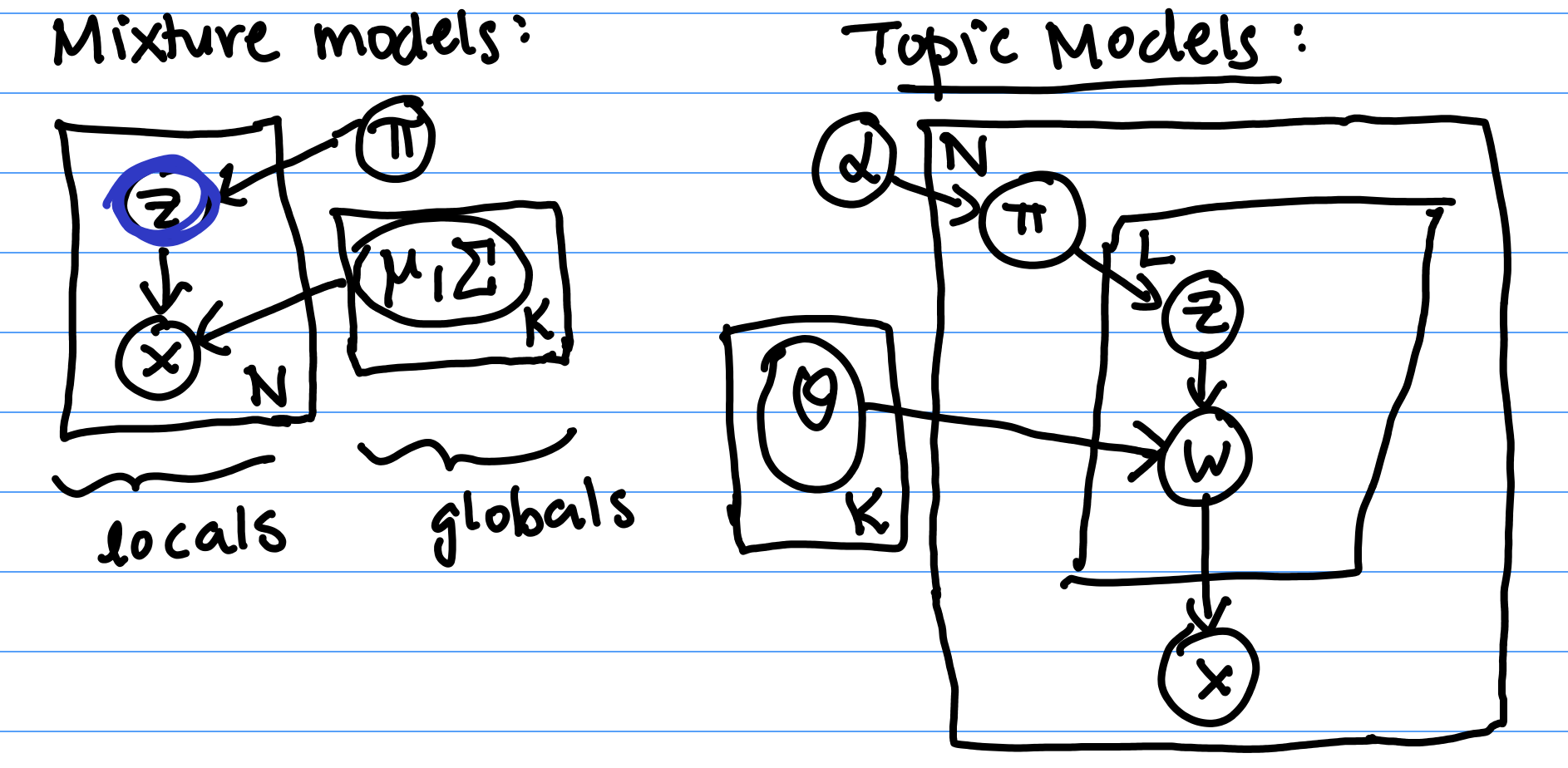
We also saw topic models, which lead to the even more complicated diagram in Figure 1 right. These diagrams help encode the structure of the data, including relationships between variables.

Notation and Rules

The notation we use in our graphical models is as follows.

1. Random variables are represented by an open circle. If we observe a random variable of a given model, then we shade it in. Otherwise, it's left open.
2. Deterministic parameters are represented by a tight, small dot.
3. Arrows indicate the probabilistic dependence relationship between different random variables and parameters. An arrow from $X$ to $Y$ means that $Y$ depends on $X$.
4. Plates, or boxes, indicate repeated sets of variables. Often there will be a number in one of the corners indicating how many times that variable is repeated. For example, if you have a training dataset of $N$ random variables $\{x_i, y_i\}_{i = 1}^{N}$ drawn from $X, Y$, you can draw a plate around $X$ and $Y$ in your model with an $N$ in the corner.

Bayesian Networks

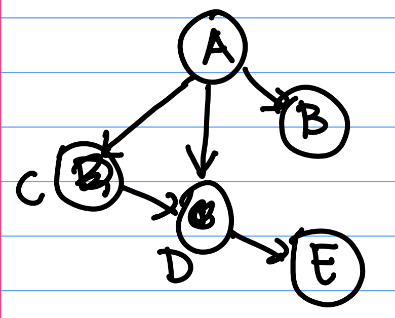
A Bayesian Network is a special kind of graphical model. Bayesian Networks (Bayes Nets) are DAGs (directed acyclic graphs) where nodes represent random variables, and directed arrows represent dependency relationships between random variables. In a DAG, nodes have directed arrows between them and there are no cycles (directed paths you can follow in a loop). In DAGS, we will be able to simplify joint probabilities nicely.

For example, the joint distribution of random variables $(A, B, C, D, E)$ can be inferred from the dependency relationships specified by the Bayes Net in Figure 2 above: \begin{align*} p(A,B,C,D,E) &= p(A)p(B|A)p(C|B,A)p(D|A,B,C)p(E|A,B,C,D) \\ &= p(A)p(B|A)p(C|A)p(D|C,A)p(E|D) \end{align*} Where the last line comes from looking at which variables depend on which other variables in the diagram. For example, C and B depend only on A, D depends on C and A, and E depends only on D. Then $ p( E | D, C, B, A)$ can be simplified to $p(E | D)$.

Why are Bayes Nets and the structure they provide useful?

1. For inference: Knowing which variables are independent helps us determine when we can use block coordinate ascent to infer their values.
2. For learning: Bayes Nets allow us to learn "smaller" distributions, or distributions with fewer parameters.
   
   For example, before the joint distribution for the network in Figure 2 is simplified, $p(E | D, C, B, A)$ is dependent on $\{A, B, C, D\}$. If each of $\{A, B, C, D\}$ is binary, then there are 16 different "settings" of $p(E | D, C, B, A)$; for example $p(E | D = 0, C = 0, B= 0, A = 0)$, $P(E | D = 1, C = 0, B= 0, A = 0)$, etc. As such, we require 16 different "parameters", or terms $p(E | D, C, B, A)$, to fully specify the distribution.
   
   However, after simplifying this term to $p(E | D)$, we only need to learn $p(E | D = 0)$ and $p(E | D = 1)$ to fully specify the distribution $p(E | D)$.
   
   

Intuition for D-separation

We will begin by defining the principle of local independence: every node is conditionally independent of its non-descendants, given only its parents.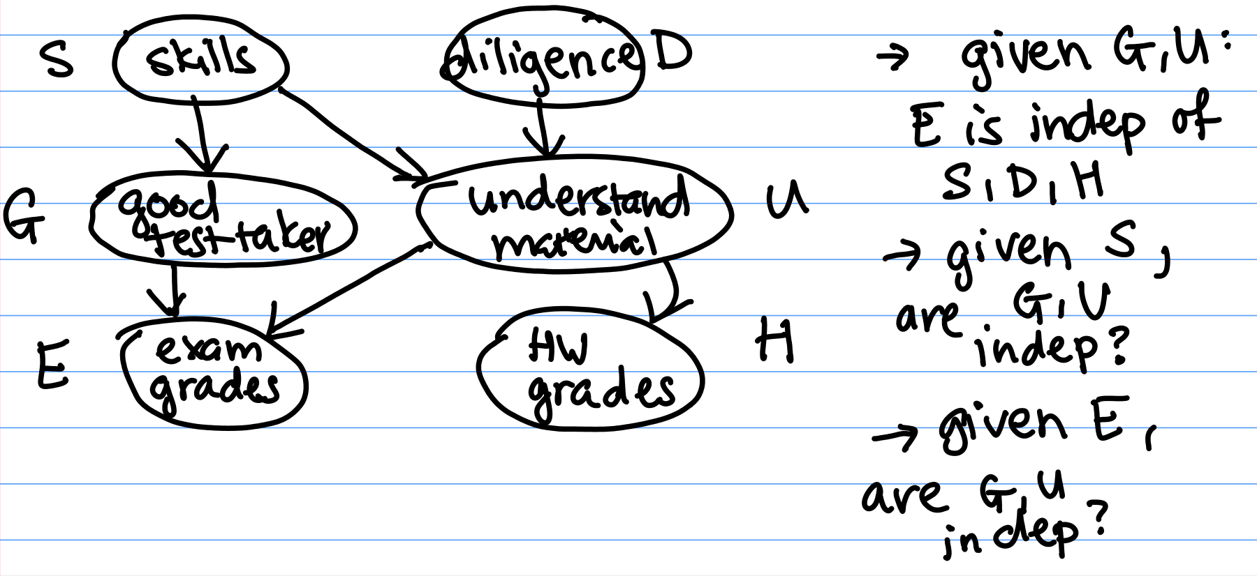

Imagine that students have skill level S and diligence D, which affect how they do in a course as shown in Figure 3. Observe that we’re using our prior beliefs about how these variables interact to bring structure to the data.

Given $G$ and $U$, $E \perp H, S, D$ (or $E$ is conditionally independent ($\perp$) of $H$, $S$, and $D$) by local independence.

Q: Given $S$, are $G$ and $U$ independent?
A: Yes: local independence says that $G$ and $U$, which are non-descendants, are independent given their parent $S$. In the graph, this means that G and U are related only through S, their parent. So given the parent, they are independent.

Q: Given $E$, are $G$ and $U$ independent?
A: No. We cannot apply the principle of local independence because $E$ is not a parent of $G$ or $U$.

Intuitively, if you know that someone did well on their exam, and you find out that they really understood the material, then you may have less idea of if they are a good test taker. Knowing that they really understood the material already “explains" their high performance on the exam. Therefore conditioned on observing the student's exam score, understanding the material and being a good test taker are dependent variables. This general phenomenon is called the explaining-away effect.

The D-separation Rules

When discussing D-separation, we use the term "information flow" to describe dependencies between variables. If there is information flowing from $A$ to $B$, then $A$ and $B$ are conditionally dependent given the observed random variables. In contrast, if $A$ and $B$ are "blocked", then $A$ and $B$ are conditionally independent given the observed random variables.

Two variables $A$ and $B$ are D-separated, or independent, if every undirected path from $A$ to $B$ is “blocked".

There are several ways a path can be "blocked":
Case 1 and 2: In Case 1, if we have observed $C$, then $B$, which is a descendant, will be independent of $A$ (by local independence). Case 2 is symmetric.

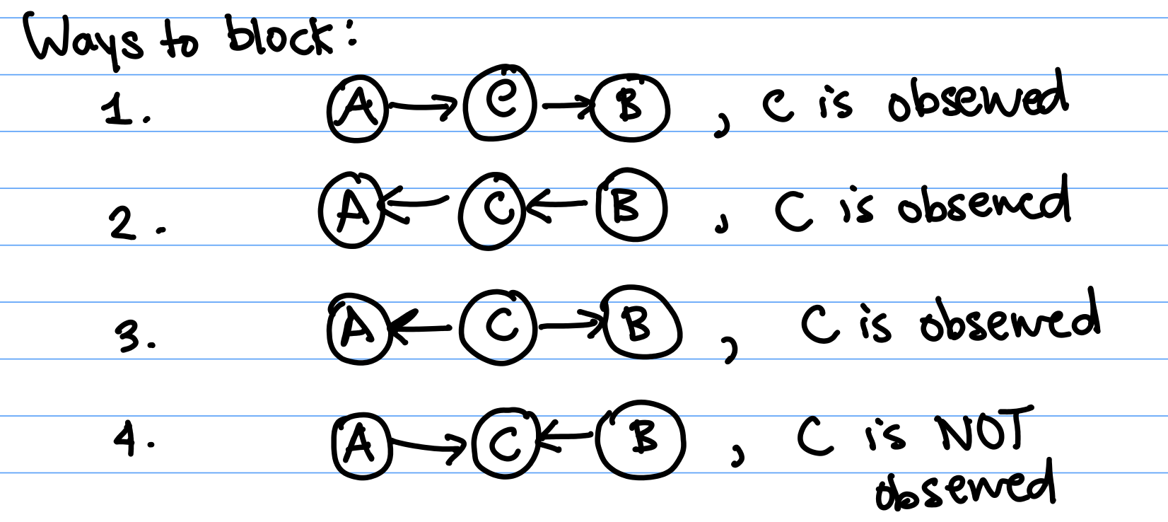
Case 3: In Case 3, $C$ is the parent of both $A$ and $B$. Because $A$ and $B$ are not descendents of each other, $A$ and $B$'s conditional independence follows by local independence.

Case 4: In Case 4, not observing C blocks the path. When C is observed, it induces a correlation, or dependency between $A$ and $B$.
Section 8.2.5 of the textbook discusses each of these D-separation rules more in-depth, we strongly recommend that you read it as a supplement to this lecture!

Uniqueness and Parameters

Uniqueness

Under a causal interpretation, A causes B and we cannot say that B causes A.

But under a statistical interpetation, instead of thinking about causal relationships, we think about how knowing the value of A can inform us about what the distribution of B is. Similarly, knowing B informs us about the distribution of A.

Given any two random variables $(A, B)$, we can write the joint distribution $p(A, B)$ two ways. Each equation has an associated "ordering", which is the direction of the arrow. $$A \longrightarrow B: p(A, B) = p(A) p(B | A)$$ $$B \longrightarrow A: p(A, B) = p(B) p(A | B)$$ A statistical interpretation allows for multiple orderings, but one ordering may require the fewest parameters and contain the most independences.

Example: Ordering affects the number of necessary parameters

Example: Recall our network from Figure 3, here written using simplified variable names: Suppose all variables are binary. How many parameters does this network need? Or, otherwise stated, how many different values do we need to know to be able to calculate the joint distribution $p(S = s, D = d, G = g, U = u, E = e, H = h)$ for all possible values $s, d, g, u, e, h \in \{0, 1\}$?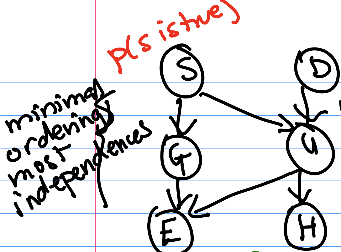

First, notice that $p(S)$ can be fully specified by $1$ parameter, as $p(S = 0) = 1- p(S = 1)$.

Similarly, $p(G | S)$ can be fully specified by 2 parameters $p(G = 1 | S = 0)$ and $p(G = 1 | S = 1)$, as $p(G = 0 | S = 0) = 1 - p(G = 1 | S = 0)$, etc. Basically, we need one parameter for each case where S came up 1 or 0. If S is 1, what’s the probability that G is 1? And if S is 0, what’s the probability that G is 1?

$p(U | S,D)$ will need 4 parameters for the 4 cases (S=0,D=0), (S=0,D=1), (S=1,D=0), (S=1, D=1) because it has 2 parents which could each take one of 2 possible values. Going on with this reasoning, E, G, and U would need 4 parameters each, and H would need 2 parameters. Then the whole network needs

$$1 + 2 + 4 + 1 + 4 + 2 = 14$$ total parameters.

Re-ordering the Network

We can change the topology (ordering) of the net, while preserving the same dependency relationships between variables. For example, the network in Figure 7 is the one from Figure 6 with a re-ordered topology, preserving the relationships from Figure 6: Say that we wish to place $E$ at the top of the network. Now, we consider $H$. Can $H$ be chosen independently of $E$ in the original network? No, because its parent $U$ (in the original network) has not been observed, so there is an unblocked path $(E, U, H)$ between them. Therefore we need an arrow from $E$ to $H$.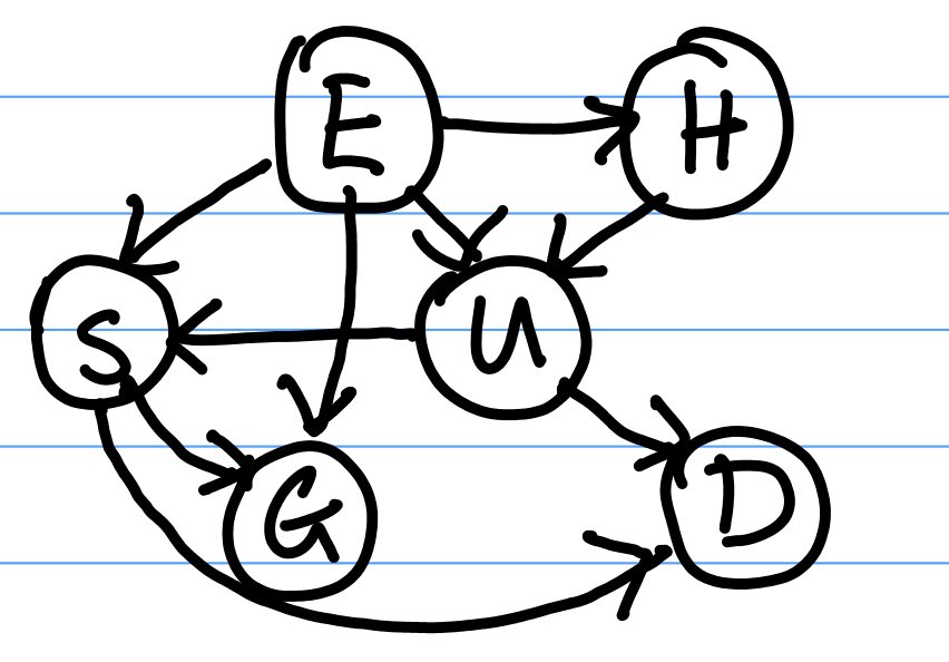

Next, we add $U$ to the new network. $U$ is not independent of $E$ or $H$, so we need to draw arrows from $E$ and $H$ to $U$.

We add $S$ to the new network. $S$ depends on $U$ and $E$ because we have not observed $G$ yet. Because $U$ has been observed, blocking all paths from $S$ to $H$, we do not draw an arrow from $H$ to $S$.

We add $G$ to the network. $G$ depends on $E$ and $S$, so we draw arrows from $E$ and $S$ to $G$.

Finally we add $D$, which depends on $U$ and $S$.

This new network respects all the dependencies of the original network. Note that the new network contains more dependencies (or arrows) than our original network.

Our new network in Figure 6 has 23 required parameters. It requires more parameters than our original network.

Beyond Bayes Nets

In CS 181, we are only going to focus on Bayesian Networks. But, there are more kinds of graphical models out there! We'll briefly introduce two other kinds of graphical models.

Undirected Models

Undirected models are graphs where the edges between random variables are undirected. For example, consider graph The joint distribution of this graph can be factored as $$P(A, B, C, D, E) = \frac{1}{z} \phi(C, A, B) \phi(B, D) \phi(B, E)$$ where $z$ is a normalizing constant and $\phi$ is a function.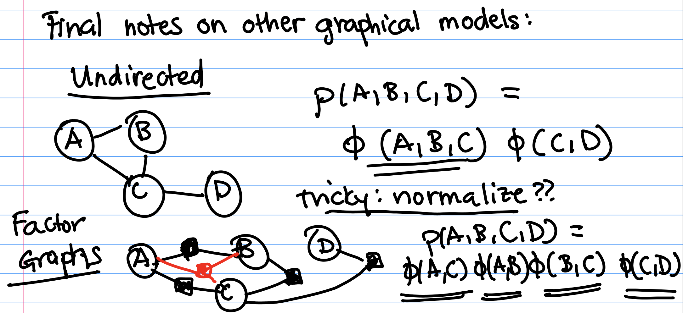

Undirected graphical models are very popular in settings such as image segmentation (you can make graphs over pixels in an image). In practice, they're hard to work with because finding the normalizing constant $z$ that makes $P(A, B, C, D, E)$ a valid probability distribution is hard.

Factor Graphs

In factor graphs, variables connect into factors, which are denoted by the shaded nodes. Each shaded node corresponds to a $\phi$: The joint distribution of the factor graph can be written as $$p(A, B, C, D, E) = \frac{1}{z} \phi(A,C) \phi(A,B) \phi(B,C) \phi(C,D)$$ where $z$ is a normalizing constant and $\phi$ is a function. Normalization here is still tricky.

Each of the $\phi()$ terms was created by examining each of the factor nodes, and including the variables which were connected to each factor.

Factor graphs are more expressive than undirected graphs. Notice here that we included a factor to add additional term $\phi(B, C)$. We wouldn't have been able to specify the inclusion of this extra term in our undirected graphical model.