Date: February 17, 2022

Relevant Textbook Sections: 4.4, 4.5, 4.6

Cube: Supervised, Discrete or Continuous, Nonprobabilistic

Lecture Video

Announcements

1. Homework deadlines have been moved from 8:00pm to 11:59pm. This means HW2 is due 11:59pm.
2. The midterm is in less than two weeks. Next Tuesday's class will be the final set of material for the midterm.

Lecture 8 Summary

• Deep Learning Today
• Deep Learning Models
• Why is this Reasonable?
• Additional Architectures

Deep Learning Today

Deep learning has been increasingly commonplace of our lifes: auto-completing words on your phone, using swipe-type, cameras automatically focussing on faces, Google translate. These tools have been only now becoming more inclusive, where automatic face focussing would only work well on people with lighter skin.

Why has deep learning been working so well? The deep learning models are entirely enabled by the massive amount of data we have access to in the modern world.

The importance of data for deep learning implies, unsurprisingly, that deep learning works well as an interpolator, but not an extrapolator.

The ideas for many deep learning models have existed since the 1990s. However, it has only been able to take off now because of the mssive computing power brought on by GPU technologies growing so rapidly in the 2010s.

Without data and without computing power, deep learning would simply not be as ubiquitous as it is today.

Deep Learning Models

Let's consider logistic regression. Recall in probabalistic classification which looked like the following $$p(y | x) = \sigma(-(w^\top x + b)) = \frac{1}{1 + \exp(-(w^\top x + b))}.$$

Given a particular slope and offset $w, b$, then the $w^\top x + b = 0$ marks the line where $p(y = 1 | x) = 0.5$. That means the boundary in logistic regression is always linear. We need a more "expressive" model class to be able to draw non-linear boundary in order to fit the structure of non-linearly seperable data.

One thing we can do is use a basis $\phi : \mathbb R^D \to \mathbb R^{D'}$ to transform the $x$. Yes, this would solve the problem by allowing us to achieve non-linear boundaries, but what if we don't know what basis $\phi$ to use? We can simply "learn" the basis. This is the fundamental idea behind deep learning. In the statistics community, deep learning is considered "adaptive basis regression".

Let $f = \mathbf w^\top \phi + \mathbf b$ and $p(y = 1| x) = \sigma(-f)$. The big question is what is the form of $\phi$? When we talk about "architecture" of a neural network, we are talking about the structure and form of $\phi$. One option is to say we have our datapoint $\mathbf x \in \mathbb R^D$ as inputs. We can then define $\phi = \sigma(\mathbf W^{(1)} \mathbf x + \mathbf b^{(1)})$ as our basis transformed datapoint where $\mathbf W^{(1)} \in \mathbb R^{J \times D}$ and $\mathbf b^{(1)} \in \mathbb R^J$. These "parameters" $\mathbf W^{(1)}$ and $\mathbf b^{(1)}$ maps $\mathbf x$ from a $D$-dimensional vector to a $J$-dimensional vector $\phi$. The superscripts indicate that these weights are done in the first step (or layer).

Why is this Reasonable?

Expressiveness

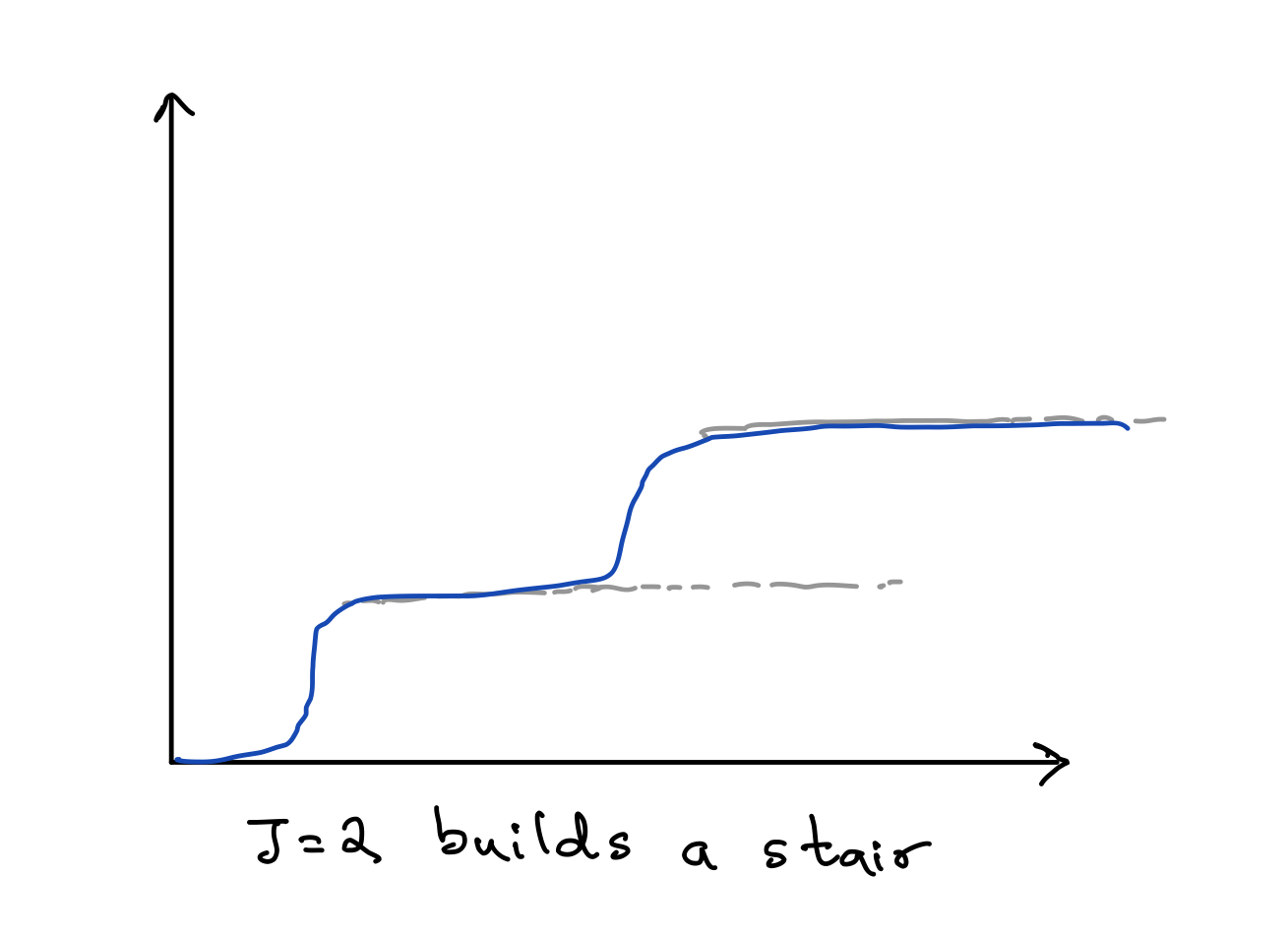
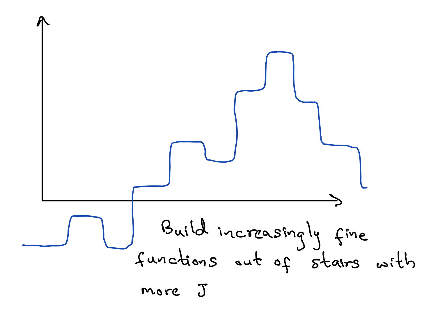
This is an expressive model class. As $J \to \infty$ gets big, this becomes a universal funciton approximator. This means we can express any function $f$. To get some intuition behind this, imagine first the J=2 scenario picking sigmoid as our activation function. Essentially, what we can do is build up a little staircase like figure below, with the sigmoid functions together. As we have more and more sigmoid functions (which we get when we add more nodes to the hidden layer), we can represent increasingly complicated functions, as if we have a really fine staircase. Notice that according to this, polynomaisl might be hard to fit with this. This relates back to inductive bias of the architecture.

Ease of Computation

The other reason why we might choose this architecture is because it is computationally easy. Computing $phi$ requires matrix multiplication and addition. It turns out that computers are great at this. This ease fascilitates both prediction and optimization.

You probably noticed that we could have changed the non-linear function we use. We call these "funcitons activation functions". Instead of using the sigmoid function $\sigma$, we could use $\tanh$ or the rectified linear unit (ReLU): $$\operatorname{RELU}(x) = \max(0, x).$$

The sigmoid activation might have an easy time representing something that looks like a set of stairs. The radial basis activation might have a easy time representing wavey functions. The ReLU activation might allow you to make jagged functions. The inductive bias is our choice of activation function and how that impacts what types of functions we can model.

Note that in classification, we will always need softmax at the end to ensure a proper probablity distribution. These function approximators can absolutely be used for regression, though!

Additional Architectures

One obvious thing we can do is add more layers. Imagine we have $L$ "hidden layers" (above, we had just one layer). Then we can say $$\Phi^{(1)} = \operatorname{a}(\mathbf W^{(0)} \mathbf X + \mathbf b^{(0)})$$ and $$\Phi^{(\ell)} = \operatorname{a}(\mathbf W^{(\ell-1)} \mathbf \Phi^{(\ell-1)} + \mathbf b^{(\ell-1)})$$ for all $1 < \ell \leq L$. Then our output would be in terms of the last hidden layer $\Phi^{(L)}$. In classification, this would look like $$\mathbf O = \operatorname{softmax}(\mathbf W^{(L)} \mathbf \Phi^{(L)} + \mathbf b^{(L)}).$$

Multiple layers allows for feature reuse which allows us to model more easily.

For state of the art architectures, we highly recommend working through the D2L.ai course.