Date: February 8, 2022

Relevant Textbook Sections: 3.6

Cube: Supervised, Discrete/Continuous, Probabilistic

Lecture Video

Lecture 5 Summary

• Motivation
• Probabilistic Classification Overview
• Discriminative Approach
• Generative Approach
• Multi-class Classification

Motivation

To motivate our exploration of probabilistic regression, let's explore some example classification problems:

• Classifying an email as spam.
• Predicting parking bans in inclement weather. What is the probability there will be greater than 5 inches of snow?
• Deciding whether or not to show a user an ad.
• Deciding whether an individual should quarantine. What is the probability an individual has COVID-19?
• Dating platform algorithms. What is the probability that person 1 will like person 2?

As illustrated in several of these examples, we often are not only interested in predicting class labels, but are also interested in approximating the probability that an example belongs to a particular class.

Recall that in last week's lecture, we used the below parametric classification model to predict label $\hat{y}_n$ as
\begin{equation} \hat{y}_n=\left\{ \begin{array}{@{}ll@{}} +1, & \text{if}\ \mathbf{w}^T \mathbf{x} + w_0 > 0 \\ -1, & \text{otherwise} \end{array}\right. \end{equation} We learn weights $\mathbf{w}$ by training using the hinge loss.

But, what if we're interested in calculating a probability that an example is positive? Today we'll discuss two approaches. In both cases, we're going to use maximum likelihood estimation to learn model parameters.

Probabilistic Classification Overview

Today we'll discuss two different approaches to probabilistic classification: the discriminative and the generative approach.

Approach 1: Discriminative

Our goal is to find parameters $\mathbf{w}$ that maximize the conditional probability of labels in the data:
$$\operatorname*{argmax}_{\mathbf{w}} \prod_n p(y_n | \mathbf{x}_n, \mathbf{w})$$ The term $p(y_n | \mathbf{x}_n, \mathbf{w})$ is called the conditional likelihood.

In this setting, the labels $y_n$ are generated based on covariates or features $\mathbf{x}_n$. We take the product in this expression because we think of individual pairs $\{(\mathbf{x}_n, y_n)\}_{n = 1}^N$ as independently and identically distributed.

We'll illustrate the discriminative approach using a method called logistic regression.

Approach 2: Generative

Our goal is to find parameters $\mathbf{w}$ that maximize the joint distribution of both the features $\mathbf{x}_n$ and labels $y_n$. $$\operatorname*{argmax}_{\mathbf{w}} \prod_n p(\mathbf{x}_n, y_n | \mathbf{w})$$ The term $p(\mathbf{x}_n, y_n | w)$ is called the joint likelihood.

In general, while the discriminative approach is simple, the generative approach is flexible. The generative approach can add knowledge and handle missing labels quite elegantly.

We'll illustrate the generative approach using two methods: multi-variate Gaussian models and Naive Bayes models.

A few notes:

• Today we will assume the two classes are $\{0, 1\}$, where $1$ is the "positive" and $0$ is the "negative" label.
• A new example $y$ has predicted label 1 if the probability that it is 1 is greater than the probability that it is 0. \begin{equation} \hat{y} =\left\{ \begin{array}{@{}ll@{}} 1, & \text{if}\ p(y = 1 | \mathbf{x}) > p(y = 0 | \mathbf{x}) \\ 0, & \text{otherwise} \end{array}\right. \end{equation}

Discriminative Approach

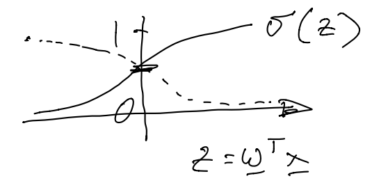
In logistic regression, we model $p(y | \mathbf{x})$ using the sigmoid (or "logistic") function: $$p(y = 1 | \mathbf{x}) = \frac{1}{1 + \exp(- \mathbf{w}^T \mathbf{x})}$$ The sigmoid (or logistic) function is often denoted using a $\sigma$, and takes scalar values as input:
$$ \sigma(z) = \frac{1}{1 + \exp(-z)}$$ The sigmoid function intuitively "flattens" its input to output values between $0$ and $1$:

In logistic regression, $p(y = 0 | \mathbf{x}) := 1 - p(y = 1 | \mathbf{x})$.

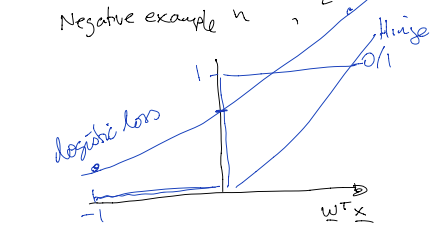
If we write $h = \mathbf{w}^T \mathbf{x}$, then $$ p(y = 1 | \mathbf{x}) = \frac{1}{1 + e^{-h}}, p(y = 0 | \mathbf{x}) = \frac{1}{1 + e^h}$$ Since $y \in \{0, 1\}$, we can rewrite $p(y | \mathbf{x})$ using the "power trick": $$ p(y | \mathbf{x}) = p( y = 1 | \mathbf{x})^y \cdot p(y = 0 | \mathbf{x})^{1 - y}$$ The parameters that maximize a likelihood function (the maximum likelihood estimate) also minimize the negative log-likelihood function. Thus, we can treat the negative log-likelihood - the expression we are minimizing - as a "loss function". Therefore the negative log-likelihood or "loss" over the dataset $D$ can be written as: $$ L_D(\mathbf{w}) = - \sum_n \ln [p(y_n | \mathbf{x}_n)]$$ Applying log rules and the power trick, $$ = - \sum_n y_n \ln [\sigma(h_n)] - \sum_n (1 - y_n) \ln [\sigma(-h_n)]$$ $$ = \sum_n y_n \ln [1 + \exp(-h_n)] + \sum_n (1 - y_n) \ln [1 + \exp(h_n)]$$ The second term $(1 - y_n) \ln [1 + \exp(h_n)]$ can be understood as the loss of the classifier on a negative example $(\mathbf{x}_n, y_n = 0)$. We can draw a picture of this logistic loss function $(1 + \exp(\mathbf{w}^T x))$. It is helpful to compare this plot of logistic loss to that of 0/1 loss and hinge loss, which we discussed last week.

The logistic loss function is differentiable and convex. This means we can use gradient descent methods to minimize this loss. Unlike the hinge loss function, the logistic loss still penalizes the classifier's predictions on data points where the classifier predicts the correct label. In a sense, logistic loss prefers to make better decisions on correct predictions, "pushing away" from the decision boundary.

Stochastic gradient descent

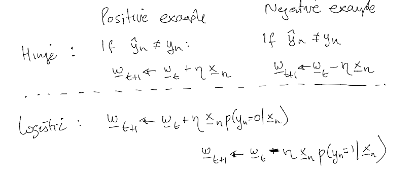
In order to use stochastic gradient descent to learn optimal parameters $\mathbf{w}$, we take the gradients of the negative log-likelihood with respect to $\mathbf{w}$. Here are the gradients with respect to $\mathbf{w}$ on examples that are true positives and true negatives for the Hinge and the logistic loss functions: When we use Hinge loss, only incorrectly classified data points contribute to the loss. But for logistic regression, even if $\hat{y}_n = y_n$, we still update parameters $\mathbf{w}_{t + 1}$.

Generative Approach

In generative classification, our goal is to model the joint distribution $p(\mathbf{x}, y)$ directly. Steps for specifying and learning a generative model are:

1. Decide on a data-generating process.
2. Choose a parametric model.
3. Minimize the negative-log likelihood.

One probability concept from probability that will be very useful when working with generative models is sometimes called the "chain" or "product" rule: $$p(\mathbf{x}, y) = p(\mathbf{x} | y) \cdot p(y)$$ Here, $p(\mathbf{x} | y)$ is called the class-conditional, and $p(y)$ is called the class prior. When we factor the joint distribution this way, this implies that labels $y$ are used to generate covariates $\mathbf{x}$. For example, if $\mathbf{x}$ are pixels in an image, and $y = 1$ if the image is of a cat, then $p(y = 1)$ is the proportion of total images that have a cat, and $p(\mathbf{x} | y)$ describes the distribution over pixel values for the images of cats.

Today, if the covariates $\mathbf{x}$ are continuous, we'll assume they are Gaussian. If they are discrete, we'll use Naive Bayes. Today we'll also assume a Bernoulli class prior.

To find the MLE of some parameters $\mathbf{w}$, first we can apply the chain rule:

$$ \operatorname*{argmax}_{\mathbf{w}} \prod_n p(\mathbf{x}_n, y_n | \mathbf{w}) = \operatorname*{argmax}_{\mathbf{w}} \prod_n p(\mathbf{x}_n | y_n, \mathbf{w}) p(y_n | \mathbf{w})$$ Transforming the likelihood into the negative log-likelihood and applying log rules, $$ \operatorname*{argmin}_{\mathbf{w}} - \sum_n \ln [p(\mathbf{x}_n | y_n, \mathbf{w})] - \sum_n \ln [p(y_n | \mathbf{w})]$$ To predict labels $y$ for covariates $\mathbf{x}$, we use Bayes' Rule: $$ p(y = 1 | \mathbf{x}) \propto p(y = 1) p(\mathbf{x} | y=1)$$

Class Prior

Today, we'll model our class prior as a Benoulli random variable with probability $\theta$. Therefore $$p(y) = \theta^y (1 - \theta)^{(1 - y)}$$ If you take $\frac{d\mathcal{L(\theta)}}{d\theta}$, then you'll find that the MLE $\theta^*$ of $\theta$ is: $$ \theta^* = \frac{\sum_n y_n}{N}$$

Class conditional with continuous $\mathbf{x}$

Say that covariates $\mathbf{x}$ are continuous. Today, let's assume that covariates are distributed as Gaussian, where the parameters of $\mathbf{x}$'s distribution differ depending on $\mathbf{x}$'s true label $y$: $$\mathbf{x} | y = 0 \sim \mathcal{N}(\mathbf{\mu}_0, \mathbf{\Sigma}_0)$$ $$\mathbf{x} | y = 1 \sim \mathcal{N}(\mathbf{\mu}_1, \mathbf{\Sigma}_1)$$ $$\mathbf{w} = \{ \mathbf{\mu}_0, \mathbf{\Sigma}_0, \mathbf{\mu}_1, \mathbf{\Sigma}_1\} $$ Intuitively, you should think of the training data $\{(\mathbf{x}_n, y_n)\}_{n = 1}^N$ as being in two piles, one for each class.

For class $0$, we use all of the data points $(\mathbf{x}_n, y_n)$ where $y_n = 0$. From these data points, we estimate $\mathbf{\mu}_0$, $\mathbf{\Sigma}_0$ for the negative class.

Similarly, we estimate $\mathbf{\mu}_1, \mathbf{\Sigma}_1$ for class $1$ using the data points with $y_n = 1$.

For example, when you derive the maximum likelihood estimate for parameter $\mathbf{\mu}_0$, you find that $$\hat{\mathbf{\mu}_0} =\frac{1}{N_0} \sum_{n: y_n = 0} \mathbf{x}_n$$ where $N_0$ is the total number of examples with label $0$. Intuitively, the MLE of the mean $\mathbf{\mu}_0$ for class $0$ is the empirical average of the covariates for all of the training data points in class $0$.

We strongly encourage you to attend section to learn more about the shape of decision boundaries learned by Gaussian generative models. If the class-conditional distributions have the same covariance matrix, then the learned decision boundaries will be linear. Otherwise, they will be quadratic.

The decision boundary for our generative model is: \begin{equation} \hat{y} =\left\{ \begin{array}{@{}ll@{}} 1, & \text{if}\ p(y = 1)p(\mathbf{x} | y = 1) > p(y = 0) p(\mathbf{x} | y = 0) \\ 0, & \text{otherwise} \end{array}\right. \end{equation}

Class-conditional with discrete $\mathbf{x}$ (Naive Bayes)

Now we will consider the case where discrete data $x_d$ takes on one of $J$ values, $\{1, ..., J\}$. For example, data $x_d$ may be hair color. If there are $10$ hair colors, then $J = 10$.

The Naive Bayes assumption is that each dimension of data $\mathbf{x}$ is independent, conditioned on the class: $$ p(\mathbf{x} | y = 1) = \prod_d p(x_d | y = 1)$$ Conditioned on class $y$, we sample hair color independently of other features (such as height).

We use Naive Bayes to limit the number of parameters needed to specify our model. If our features were dependent on each other, then we would need to explicitly model this dependence using additional parameters.

We model each feature $x_d$ as a categorical distribution. The categorical is a generalization of the Bernoulli distribution. For example, if there are 3 hair colors (blonde, black, and brown), then vector $\pi_{dk} = [\pi_{dk1} = 0.2, \pi_{dk2} = 0.5, \pi_{dk3} = 0.3]$ parameterizes $x_{dk}$, where we use notation $$ \pi_{kdj} \geq 0$$ where $\pi_{kdj}$ is the probability in class $k$, of feature $d$ taking on value $j$.

You can now do a maximum likelihood fit of parameters $\pi_0$ for class $0$, and $\pi_1$ for class $1$. Similarly here we use the class $0$ data to estimate the parameters $\pi_0$, and the class $1$ data to estimate the parameters $\pi_1$.

Notes:

• In this discrete case, our Naive Bayes classifier has linear decision boundaries.
• In this course, we often use the notation $C := \{C_1, ..., C_k\}$ to denote the $k$ classes $C_1$, $C_2$, etc.

Multi-class Classification

How do we move from binary to multi-class classification?

In the generative setting, it's easy: just use a categorical class prior and estimate class conditions. Classify as $$ \operatorname*{argmax}_{k} p(\mathbf{x} | y_k) p(y_k)$$ In a discriminative setting, we need to have separate parameters $\mathbf{w}_k$ for each class. We classify using the "softmax" function: $$p(y = C_k | \mathbf{x}) = \frac{\exp(\mathbf{w}_k^T \mathbf{x})}{\sum_{k=1}^K \exp(\mathbf{w}^T_k \mathbf{x})} $$ Because of the normalizing denominator term $\sum_{k=1}^K \exp(\mathbf{w}^T_k \mathbf{x})$, the "softmax" probabilities sum to 1 across classes $k$: $$\sum_{k = 1}^K p(y = C_k | \mathbf{x}) = \sum_{k=1}^K \frac{\exp(\mathbf{w}_k^T \mathbf{x})}{\sum_{k=1}^K \exp(\mathbf{w}^T_k \mathbf{x})} = 1$$ To learn non-linear decision boundaries, we can apply basis functions to our data. See the lecture slides for visualizations.