Date: March 10, 2022

Relevant Textbook Sections: 6

Cube: Unsupervised, Discrete, Nonprobabilistic

Lecture Video

Announcements

1. HW3 is due this Friday.
2. HW4 is released tomorrow, but it designed to take a week.
3. Enjoy the break!

Relevant Videos

• K Means
• HAC

Summary

• Intro to Unsupervised Learning
• Nonprobabilistic Clustering: K-Means
• Nonprobabilistic Clustering: Hierarchical Agglomerative Clustering

Intro to Unsupervised Learning

So far in the class, we've been doing supervised learning, where we try to predict y's (labels) given x's (data). Now, we'll look at unsupervised learning, where there are no more y's, and only x's. Instead of labeling the data, the task is now to "summarize" the data. At the most general level, unsupervised learning is a "summarization task" that we're trying to complete. This is helpful for:

1. Figuring out what classes or labels to later use with this data in a supervised learning model
2. Compressing high-dimensional data, like images, to lower dimensions in order to save storage space
3. Organizing data, like grouping news articles covering the same topic or songs with the same style together

Today we’ll cover clustering, a method for putting data into groups.

Nonprobabilistic Clustering: K-Means

Scenario and Notation

First, we define our K-means clustering problem.

• We have our data $x_1, x_2, ..., x_n$
• We may be given a number $K$ of desired clusters to find
• We want an algorithm that outputs group assignments $z_{nk}$, where $z_{nk}$ tells us if $x_n$ is in cluster $k$. That is, $$ z_{nk} = \begin{cases} 0 & x_n \text{ is not in cluster } k \\ 1 & x_n \text{ is in cluster } k \end{cases} $$

Intuitively, we want to split the data into K clusters so that examples are similar to other members of their same cluster, but not similar to the members of other clusters. To accomplish this, we’ll need some way to measure how different two datapoints are. We have a number of options; we could use Euclidean distance, edit distance for text data, or Hamming distance. For today, we will just use Euclidean distance: $$d(x, x') = ||x - x'||_2.$$ For K-means clustering, the point $\mu_k$ will be a "prototype" of the cluster $k$. The idea is that $\mu_k$ defines cluster $k$ by representing its center point. Note: $\mu_k$ should have the same dimensions as each datapoint $x_i$.

The Objective

We use the following objective for the K-means problem. The idea is that we want to find the $\mu$’s (cluster centers) and $z$’s (cluster assignments) so that data points $x_n$ are close to the centers of the clusters they got assigned to. $$\min_{z, u} \sum_n \sum_k z_{nk} ||x_n - \mu_k||_2^2 $$ Recall that $z_{nk}$ is either 0 or 1 depending on if $x_n$ is in cluster $k$. In the sum, we multiply the distances by $z_{nk}$ so that only distances from $\mu_k$ to points in cluster $k$ count in our loss. This is just like how we've used indicator variables in the past.

It turns out this optimization is NP hard and non convex, so it's difficult to solve. Luckily, Lloyd’s algorithm helps us find a pretty good local optimum.

Lloyd's Algorithm

We can find clustering assignments for K-means by following this algorithm:

1. Randomly initialize prototypes $\mu_k$
2. Repeat until converged:
1. Assign each example to its closest prototype $$x_n = \textrm{argmin}_k ||x_n - \mu_k ||_2$$
2. For each cluster $k$, set $\mu_k$ to the centroid (mean) of the examples assigned to this cluster $$\mu_k = \textrm{mean}(x_n\textrm{ such that }z_{nk} = 1) = \frac{1}{N_k} \sum z_{nk} x_n,$$ where $N_k$, the number of items in the cluster, is obtained by $\sum_n z_{nk}$

The results of this algorithm depend on how the prototypes are initialized. Usually, we restart it several times and pick the best solution found.

This idea of alternating optimization (aka coordinate descent) is going to be key in our unsupervised learning, because now we have two sets of unknowns to find, the global $\mu$’s and the data-specific z's).

Why Lloyd's Algorithm Works

At a high level, this algorithm works because in each step (the calculating z step, and the calculating $\mu$ step), we are reducing the loss. Since we are doing this until convergence, we will reach some local minimum.

For calculating z:

When we calculate the $z$’s, we are assigning each point to the cluster with the closest prototype. Of course this is the choice that would minimize loss for the current locations of prototypes, as we are shortening (or not changing) the distance between points and their prototypes.

For calculating $\mu$:

We can go back to the objective function and set its derivative with respect to $\mu_k$ to 0 to show that the step we take in Lloyd's algorithm minimizes the loss. $$L = \min_{z, u} \sum_n \sum_k z_{nk} ||x_n - \mu_k||_2^2 = \sum_n z_{nk} (x_n - \mu_k)^T(x_n - \mu_k)$$ We can take this derivative with respect to $\mu_k$. $$\frac{\partial L}{\partial \mu_k} = - 2 \sum z_{nk} (x_n - \mu_k) = 0$$ $$\left ( \sum_n z_{nk} \right )\mu_k = \sum_n z_{nk} x_n$$ We pulled out the $\mu$ since it doesn't depend on n. $$\mu_k = \frac{\sum_n z_{nk} x_n}{\sum_n z_{nk}} = \frac{\sum_n z_{nk} x_n}{N_k}$$ This is exactly what we set $\mu_k$ to when running our algorithm, illustrating how the algorithm finds a local minimum for $\mu$.

Selecting K

How many clusters should we pick? We plot the lowest loss achieved for different values of K and look for the value of K corresponding to a bend in the loss curve. This is also known as the elbow method. The idea is that as we increase K, the loss will keep decreasing. In fact, if we set K to be as big as n, the number of data points we have, each point can be its own cluster and the loss will be 0. So it doesn’t make sense for us to minimize the loss. Instead, we look to see where the plot of loss vs. clusters makes an elbow shape - this is when the improvement in loss levels off as we add more clusters, and the returns on adding more clusters are diminishing.

More Comments About K-Means

• K-means is a parametric method, where the parameters are the prototypes.
• Inflexible; the decision boundary is linear.
• Fast! The update steps can be parallelized.
• There are several variations on the basic K-means algorithm
1. K-means++ gives a more specific way to initialize clusters
2. K-medoids chooses the centermost datapoint in the cluster as the prototype instead of the centroid. (The centroid may not correspond to a datapoint.)

Nonprobabilistic Clustering: Hierarchical Agglomerative Clustering

The Algorithm

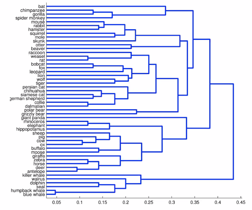
The Hierarchical Agglomerative Clustering (HAC) algorithm is as follows:

1. Every example starts in its own cluster.
2. While there is more than 1 cluster, we merge the two “closest” clusters.

This forms a hierarchy of clusters, which can be visualized as a dendrogram (a tree) over the data where nodes are clusters, and a node $x$’s children represent the clusters that were at one point merged into node $x$.

Some features of HAC include:

• HAC is nonparametric
• It is also deterministic because there is no random intialization involved
• We do not need to specify a number of clusters to find
• Complexity scales as $O(Tn^2)$, where T is the number of iterations (merges) used, because the algorithm is based off of pairwise distance comparisons. If we merge until all clusters are combined, T will be $O(N)$.

Distance Between Points and Distance Between Clusters

For HAC, we need two measures of distance:

• $d(x, x’)$ will measure the distance between individual points
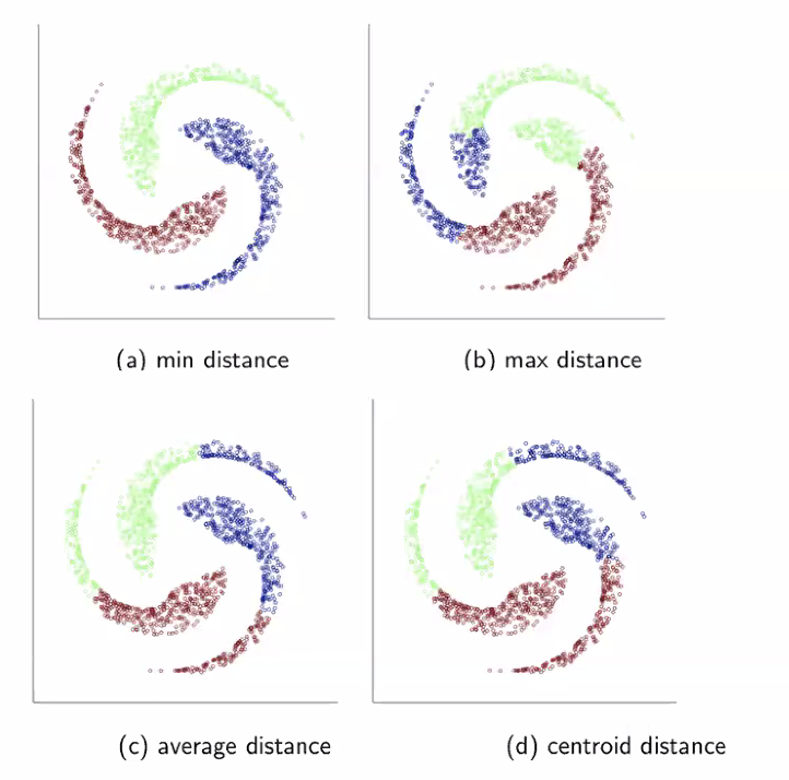
• A linkage function will measure the distance between two clusters of points. This is how we determine what the "closest" pair of clusters are. Some options for the linkage function are
• Minimum distance between two elements of the clusters (where "distance" here is measured by our distance function $d$)
• Maximum distance between two elements of the clusters
• Average distance between elements in the different clusters
• Distance between the centroids of the clusters

The min linkage is more likely to merge large clusters together, as there will be a greater chance of some element of cluster A being close to some element of cluster B when A and B are large. The min linkage will also tend to merge clusters into “chains” or “strings”. The max linkage will prefer compact clusters instead. The average and centroid linkages are compromises between the min and max ones. You will need to pick a linkage depending on what you want your output to look like.